
October 2026
Transformer architectures dominate sequence modeling across natural
language processing, computer vision, speech, and computational biology,
but the design space around them has fragmented. Attention has
diversified beyond dense softmax into recurrent and retentive blocks,
sparse patterns, gated mechanisms, latent projections, memory-augmented
layers, and fast-weight rules; optimizers have expanded beyond AdamW
with variance-reduction, memory-efficient, schedule-free, second-order,
and low-rank methods. Comparing these ideas under consistent conditions
remains costly, because each variant must be implemented, wired into a
training pipeline, and maintained separately—a duplication of effort
that hinders reproducibility and makes published comparisons difficult
to align. We present Frankenstein Transformer, a configuration-driven
CLI toolkit (frankenstein-transformer) that unifies model
definition, training, deployment, and inference behind a single strict
YAML schema. The toolkit covers fifty sequence mixers across nine
families and thirty-eight optimizer families with per-parameter-group
hyperparameter control, and supports encoder, decoder, Vision
Transformer and audio model classes for masked language modeling, causal
language modeling, sentence embeddings, image tasks, speech recognition
and audio classification. Its contribution is a validated
experimentation contract: invalid configurations fail before training
starts, every architecture and optimizer shares one operational
interface, and the same document drives training, quantized deployment
and export, and a schema-generated web builder. The contract is
exercised end-to-end in a measurement campaign of 868 configurations
(905 CPU-hours) that trains, exports, quantizes, and evaluates every
mixer pair, optimizer, and deployment path through the same interface,
published as an interactive report with downloadable datasets. We
describe the architecture taxonomy, optimizer routing, deployment paths,
and integration surface, and defer mathematical and implementation
detail to the appendices.
Transformer architectures are the dominant paradigm for sequence modeling in natural language processing , computer vision, and computational biology, with models such as BERT and GPT establishing the standard for representation learning. The field has since diversified rapidly: recurrent and retentive blocks, sparse attention, gated mechanisms, latent projections, memory-augmented layers, fast-weight rules, and continuous-depth formulations each address a different limitation of dense attention, while the optimizer landscape has expanded beyond AdamW with variance-reduction, memory-efficient, schedule-free, second-order, and low-rank methods .
The practical consequence is a fragmented ecosystem. Comparing sequence mixers or optimizers under identical training conditions requires re-implementing each variant, wiring it into a training pipeline, and maintaining the result across framework changes. This effort hinders reproducibility, slows scientific progress, and raises the barrier to entry for new researchers.
We propose Frankenstein Transformer (https://github.com/erickfmm/frankenstein-transformer), a configuration-driven toolkit that treats architecture, optimizer, and training choices as a single validated document. The project provides:
Schema-first design: a strict YAML contract supporting fifty-six sequence mixers across nine families and thirty-eight optimizer families, enforced before training begins.
Architecture-agnostic training: one pipeline for dense baselines, recurrent and retentive blocks, sparse patterns, gated mechanisms, latent compression, memory layers, fast-weight attention, and geometric-field attention, with encoder and decoder modes .
Optimizer routing: prefixed hyperparameter groups that control embeddings, normalization layers, attention blocks, and remaining parameters independently for each optimizer family .
End-to-end workflows: training (including sentence-embedding objectives), deployment and export (quantized, standard, HuggingFace safetensors at 8/4/2 bits, and BitNet GGUF formats), inference, and a schema-driven web builder inspired by SBERT-style workflows .
Vision support: a Vision Transformer model class covering masked patch prediction, classification, and segmentation under the same mixer and optimizer infrastructure.
Validation tooling: unit tests, YAML preset validation, and continuous integration across supported Python versions.
The command surface is frankenstein-transformer, with
four subcommands: train, deploy,
infer, and web-server. The last launches a
Streamlit configuration builder that renders schema metadata as forms,
validates input live, previews the resulting YAML, and generates the
equivalent CLI command, serving both as a configuration aid and as
documentation of the available design space; a hosted instance runs at
https://erickfmm.github.io/frankenstein-transformer/index.html.
This document is organized as a technical reference:
Prerequisites: Appendix 12 introduces transformers and attention for readers new to the field.
Configuration contract: Section 3.1 describes the schema and Section 3.2 its validation rules.
Architecture selection: Section 4.1 compares sequence-mixer families; Appendices 13, 14, 15, and 16 collect the supporting literature, with normalization details in Appendix 21, BitNet quantization in Appendix 22, and conditional-memory details in Appendix 24, and manifold-constrained residuals in Appendix 27.
Optimization: Section 5 summarizes optimizer routing; Appendix 20 provides the full family analysis.
Deployment and inference: Sections 6 and 7 cover quantized deployment and sentence embeddings.
This work sits at the intersection of deep learning frameworks, training tooling, and configuration-driven experimentation. While Sections 4.1 and 5 survey the architectural and optimization literature in depth, this section focuses on the software ecosystem for building, training, and configuring transformer models.
The modern transformer research ecosystem rests on several foundational frameworks that provide automatic differentiation, GPU acceleration, and high-level model-building APIs.
PyTorch has become the dominant
framework for transformer research. Its imperative programming model and
dynamic computation graphs enable flexible debugging and rapid
prototyping of novel architectures. The torch.nn.Module
abstraction, automatic mixed-precision training via
torch.cuda.amp, and the torch.compile JIT
compiler form the backbone of most contemporary transformer
implementations. Frankenstein Transformer is built entirely on PyTorch,
leveraging its module system for composable architecture
definitions.
TensorFlow pioneered production-oriented
deep learning with its static computation graph paradigm and the Keras
high-level API. While its influence in transformer research has waned
relative to PyTorch, TensorFlow’s serving infrastructure
(TF Serving, TF Lite) and the
tensorflow-text library remain relevant for deployment
scenarios.
JAX offers a functional programming
model built around composable transformations (jit,
vmap, grad) and XLA compilation. Its design
enables clean implementations of complex algorithms and has been adopted
by several recent transformer libraries (e.g., Flax, Haiku). JAX’s
stateless design and automatic vectorization are particularly
well-suited for research on novel attention mechanisms and optimization
algorithms.
scikit-learn provides classical machine learning algorithms and utilities (preprocessing, metrics, model selection) that serve as baselines and complementary tools in transformer workflows. While not designed for deep learning, its consistent API and extensive documentation make it a standard reference point for comparing transformer-based approaches against traditional methods.
Several libraries provide complete training pipelines that abstract away the complexity of distributed training, data loading, and hyperparameter management.
Hugging Face Transformers is the de facto standard for
accessing, fine-tuning, and sharing pretrained transformer models. Its
Trainer API, model hub with over 500,000 models, and tight
integration with the datasets and tokenizers
libraries have made it the primary entry point for transformer-based
NLP. However, its architecture is optimized for fine-tuning existing
pretrained models rather than experimenting with novel sequence mixer
designs or training from scratch with custom optimization
strategies.
Oumi (https://github.com/oumi-ai/oumi, 2025) is
an open-source end-to-end platform for training, fine-tuning,
evaluating, and deploying foundation models. It provides a unified
interface across multiple cloud providers and supports both supervised
fine-tuning and preference optimization (DPO, RLHF). Oumi emphasizes
production readiness with built-in monitoring, checkpointing, and
deployment tooling.
LLaMA Factory (https://github.com/hiyouga/LLaMA-Factory,
2024) offers a unified framework for efficient fine-tuning of over 100
large language models. It provides both a web-based UI and a CLI,
supporting LoRA, QLoRA, full-parameter fine-tuning, and various
alignment techniques. Its focus is on adapting existing pretrained LLMs
to downstream tasks rather than architectural experimentation.
Axolotl (https://github.com/axolotl-ai-cloud/axolotl,
2024) is a streamlined fine-tuning tool supporting LoRA, QLoRA,
DeepSpeed, and FSDP. It emphasizes configuration-driven workflows via
YAML files and has become popular in the open-source LLM fine-tuning
community. Like LLaMA Factory, it targets fine-tuning of pretrained
models rather than training novel architectures from scratch.
A growing category of tools prioritizes accessibility and computational efficiency, lowering the barrier to transformer training.
Unsloth (https://github.com/unslothai/unsloth, 2024)
provides low-code fine-tuning with 2–5\(\times\) speedup and significantly reduced
VRAM requirements through hand-written CUDA kernels and optimized Triton
operations. It supports GGUF export for quantized deployment and
integrates with the Hugging Face ecosystem. Unsloth’s focus is on making
fine-tuning faster and more memory-efficient, not on architectural
exploration.
dashAI (https://github.com/DashAISoftware/dashAI,
v0.9.7.post2, 2026) is an open-source, local-first desktop workbench for
machine learning developed by a Chilean academic consortium (Universidad
de Chile/FCFM, CENIA, IMFD, and ANID funding). Its interface is fully
schema-driven: configuration forms are generated directly from Pydantic
component schemas with no hand-written frontend code, and its catalog
spans roughly 76 multitask models—tabular classifiers, NLP models,
translation, open-weight LLMs, and text-to-image generation—unified
behind a dozen typed base abstractions. Extensibility is central to its
design: plugins are ordinary PyPI packages discovered through the
dashai.plugins entry-points group and installable from the
UI, a mechanism comprehensive enough that even dashAI’s own generative
capabilities (e.g., Stable Diffusion, Flux) are distributed as plugins.
Where earlier releases targeted classical ML workflows, the current
platform spans predictive and generative modeling across domains, making
it a natural host for transformer components via its plugin system;
Section 8 presents the
dashai-frankenstein adapter built on this mechanism.
A common thread across the tools surveyed above is their focus on fine-tuning existing pretrained models. Hugging Face Transformers, LLaMA Factory, Axolotl, and Unsloth all assume a pretrained checkpoint as the starting point. Oumi supports training from scratch but targets standard architectures. None of these tools provide a systematic framework for experimenting with novel sequence mixer architectures, comparing diverse optimization algorithms under controlled conditions, or exploring the interaction between architectural choices and training dynamics.
Frankenstein Transformer fills this gap by providing a schema-first configuration system purpose-built for architecture experimentation. Its key differentiators include:
50 sequence mixers spanning dense attention, recurrent/retentive blocks, sparse attention patterns, gated mechanisms, latent compression, memory layers, fast-weight attention, and geometric-field attention, all selectable via a single YAML field.
23 optimizer families with a prefixed hyperparameter routing system that enables per-parameter-group control across embeddings, normalization layers, attention blocks, and feed-forward networks.
Dual training modes supporting both encoder-style masked language modeling (MLM) and decoder-style autoregressive (AR) next-token prediction, with specialized fine-tuning workflows for each.
Strict schema validation via
additionalProperties: false constraints that prevent
configuration errors before training begins, ensuring reproducibility
across experiments.
End-to-end workflows spanning quantized deployment (ternary weight packing, INT8 activations) and sentence-embedding training inspired by SBERT .
Web-based configuration interface providing schema-driven form rendering with inline documentation, real-time validation, and CLI command generation.
By decoupling architecture definition from training infrastructure through a validated configuration contract, Frankenstein Transformer enables systematic comparison of sequence mixer families and optimization strategies under identical training conditions—a capability not provided by any existing tool in the ecosystem.
Experimentation in this project is schema first. Rather than exposing loosely checked flags, model topology, optimizer family, training limits, and telemetry pass through a single validated configuration document, which reduces ambiguity when reproducing results and lets many architectures share one operational interface.
The authoritative contract is , a modular JSON Schema whose modules
under cover the model, model class, tokenizer, optimizer, SBERT,
training, and dataset blocks. The top-level objects are
base_model, tokenizer,
model_class, model, training,
image, vision_dataset, audio,
audio_dataset, text_dataset,
inference, and plugins.
The model_class field selects among three variants:
frankenstein_text_encoder:
mixed-architecture encoder with the full range of sequence mixers, MoE,
and advanced normalization, trained with masked language
modeling.
frankenstein_text_decoder:
autoregressive causal decoder for next-token generation; the runtime
forces decoder masking.
frankenstein_vit: Vision
Transformer over image patches for masked patch prediction,
classification, and segmentation; the runtime forces encoder masking and
the configuration requires the image and
vision_dataset blocks.
model.dims.mode controls masking: encoder
uses bidirectional attention for masked language modeling, and
decoder uses causal masking for autoregressive
prediction.
The runtime configuration mirrors the validated document one-to-one:
the nested model: block is materialised as a typed
configuration tree and per-component knobs are bound through the
component’s declarative record, with no nested-to-flat rewriting stage.
Every pluggable component—sequence mixer, optimizer, normalization,
activation, residual strategy, positional encoding and token-embedding
variant—is described by one registry entry holding its name, lazily
imported implementation, parameter schema fragment, runtime defaults,
capability flags (KV-cache support, training-time sparsity,
QK-normalization support, gated-FFN status) and bilingual documentation.
The schema enumerations, per-mixer parameter objects, optimizer prefix
reference and conditional prefix rules are assembled from that
registry before validation, so a component is declared once and
cannot drift across parallel lists; the closed-world validation
guarantee (additionalProperties: false) holds for every
registered component. The same mechanism is the extension surface: a
plugin module registers new components through a public authoring API,
either listed under the configuration’s plugins: key or
discovered through the frankenstein.plugins entry-point
group. Plugin-declared components therefore validate strictly, appear in
the schema-generated web builder, and are dispatched by the same core
code as the built-ins, while a plugin that does not declare KV-cache
support simply falls back to the full-recompute path (decision D5).
model.dims.layer_pattern is an ordered list of mixer
identifiers drawn from the eight families described in Section 4; the schema fixes the
accepted identifiers, and the complete enumeration appears in Figure 2 and Appendix 38.
training.optimizer.optimizer_class selects one of
thirty-eight optimizer families, summarized in Section 5 and detailed in
Appendix 20.
Top-level and nested objects set
additionalProperties: false, so unknown keys fail fast
instead of being silently ignored. Optimizer parameters are further
constrained by per-family prefix rules. Cross-component validation
rejects incompatible combinations before training: hidden size must be
divisible by the number of heads, the number of key–value heads must
divide the number of heads, vocabulary size must match the tokenizer, a
base model requires a task and (for MLM) a tokenizer, each task requires
its matching optimizer block, BitNet router flags require BitNet to be
enabled, and the decoder and vision classes force their respective
masking modes.
The complete schema—fields, types, ranges, and validation rules—is
documented in Appendix 37.
Looped blocks are configured through num_layers and
num_loops, giving num_layers\(\times\)num_loops logical
layers at fixed parameter count.
training.task selects the objective: mlm
(masked language modeling), causal_lm (autoregressive
next-token prediction, decoder class only), sbert (sentence
embeddings), text_classification (encoder class only), and
the vision tasks patch_prediction,
classification, and segmentation (Vision
Transformer only). NLP tasks consume text_dataset; vision
tasks consume vision_dataset. Sentence-embedding workflows
are described in Section 7.
The training step accumulates gradients over micro-batches, clips the
global norm, checks for post-clip overflow, retries a bounded number of
times on non-finite values, dispatches the configured scheduler, and
rotates rolling and best checkpoints. When
training.test_percentage is positive, a deterministic
fraction of the dataset is held out before training and the final
weights are evaluated on it; the loss and task accuracy (character error
rate for ASR) are written to test_metrics.json. A single
training.seed (default \(42\)) controls the run’s randomness: it
seeds the Python, NumPy, PyTorch and CUDA generators, model weight
initialization, DataLoader shuffle generators and workers, and the
held-out permutation, and it enables deterministic cuDNN, so repeated
runs on the same hardware and software stack reproduce initialization,
batch order and split. The full pseudocode and the split formulation are
deferred to Appendix 24.
Normalization is both a modeling choice and a schema compatibility
question. The accepted norm.type values are
layer_norm, dynamic_tanh, derf,
rms_norm, prms_norm (partial RMSNorm), and
flash_norm (weightless RMSNorm). Their formulations and
comparison are detailed in Appendix 21.
Residual connections are exposed as a macro-design choice through the
model.residuals block:
Standard: the classical identity residual .
None: no skip connection, retained only as an ablation probe.
Attention Residuals (full_attn or
block_attn): learned attention over depth replaces the
fixed residual sum, either over all previous layers or over block-wise
summaries .
Manifold-constrained hyper-connections
(mhc.enabled): an \(n\)-stream residual whose mixing matrix is
constrained to the Birkhoff polytope .
Attention Residuals compose with mHC and Mixture-of-Depths; the formulations, wiring, and reported results are collected in Appendices 28 and 27.
The system implements fifty-six sequence mixers organized into nine functional categories that reflect how each method balances expressivity, computational cost, and memory.
Dense baselines (6): standard softmax attention, sigmoid attention, Continuum Attention, Grouped-Query Attention (GQA), Exclusive Self Attention (XSA), and Multi-Token Attention (MTA) provide full global routing at quadratic cost. XSA keeps the standard softmax block and strips the component of each head’s output along the token’s own value vector , a parameter-free exclusion that sharpens the division of labor between attention and the feed-forward path.
Recurrent and retentive (3): RetNet, Mamba, and ODE-style blocks maintain state for constant-time inference through recurrence, selective state spaces, or continuous depth.
Sparse patterns (11): Sparse Transformer, Longformer, SWA with attention sinks, BigBird, SparseK, NSA, SpargeAttn, FASA, MSA, SparDA, and LSA reduce quadratic cost through structured sparsity, token selection, training-free pruning, or semantic key clustering.
Gated mechanisms (9): GLA, DeltaNet, Gated DeltaNet, Gated DeltaNet-2, HGRN2, FoX, Gated Softmax, KDA, and First Passage Attention (FPA) introduce data-dependent control over retention, forgetting, and update strength.
Latent compression (13): MLA, GQLA, MLRA, Tucker, KPA, TPA, MFA, IHA, GTA, MTLA, CCA, CCGQA, and GMA compress key–value state into low-rank bottlenecks or route through a Gaussian-mixture latent memory.
Memory (3): Titans pairs a local attention window with a surprise-driven associative memory updated at test time, Engram provides test-time read/write memory through learned N-gram hash lookups, and Memory Attention replaces the dedicated value projection with a layer-specific token-ID table.
Fast-weight attention (6): Falcon-1/2/3 and Falcon-1A/2A/3A treat the recurrent state transition as an online continual-learning rule .
Geometric field (1): SSOG applies a structured geometric prior over the attention matrix .
Convolution-augmented (2): the Conformer block fuses multi-head self-attention with a depthwise-convolution module between two Macaron feed-forward layers, giving every layer a local branch alongside the global receptive field; Fast Conformer keeps that design for long-form speech and replaces global self-attention with a limited local window plus a head-pinned global token (Appendix 19).

The dense baselines—standard softmax , sigmoid attention , and Continuum Attention , which replaces the softmax with exact integration of an exponential relevance density over piecewise-linear key/value trajectories—and the recurrent family—RetNet , Mamba , and ODE-style blocks —define the expressiveness-versus-efficiency trade-off. Formulations, parallel and recurrent forms, pseudocode, and a comparison table are collected in Appendix 13.


The memory family groups three mechanisms that add storage beside the attention operator. Titans runs dense attention over a local window while a surprise-driven associative memory is updated at test time; this repository implements the attention window only, and the neural-memory module is not part of the implementation. Engram retrieves N-gram embeddings through per-order hash tables and gates them into the residual stream. Memory Attention keeps the standard softmax attention operator but removes the dedicated value projection: values are the contextual keys plus a layer-specific, token-ID-indexed memory row, \(V = K + \mathrm{Norm}(E[s])\), with RoPE applied only to the scoring pair. It increases parameter capacity without proportional dense computation and retains a conventional KV cache at inference.

This family compresses per-token key–value state into a low-rank latent: MLA, GQLA, MLRA, Tucker, KPA, TPA, MFA, IHA, GTA, and MTLA unify grouped-query, latent, Kronecker- and CP-factorized, and temporal designs. CCA and CCGQA formulate attention in a compressed latent with decoupled grouping, while GMA replaces pairwise interaction with probabilistic routing through learned Gaussian-mixture components. Formulations, pseudocode, and a comparison table are collected in Appendix 14.

The registry includes twelve sparse blocks .
Two inference-time methods, fasa and sparge,
apply their sparse heuristic only when the model is in evaluation mode:
during training the enclosing hybrid layer substitutes standard dense
attention over the same \(\mathbf{q}/\mathbf{k}/\mathbf{v}/\mathbf{o}\)
projections, so the trained weights are exactly the ones the sparse path
reads at inference. swa is also training-free but is a
normal trainable mixer, so it runs its windowed pattern in both training
and inference. LSA is the family’s semantic selector: keys are pooled
and Ward-clustered per 512-token block, and each query scores the cached
bucket centroids instead of every key, selecting top-\(p\) buckets that expand into its \(k\) long-range keys on top of sinks and a
one-block window. ProbSparse
inverts the axis: it ranks queries with a max–mean approximation of the
KL divergence against the uniform distribution over a sampled key subset
and scores only the top-\(u = c_2\lceil\ln
L\rceil\) dominant ones, which brings the layer to \(\mathcal{O}(L\log L)\) for long
bidirectional encoders while leaving decoding dense. Formulations,
pseudocode, per-block characteristics, and a comparison table are
collected in Appendix 15.

The gated family contains nine blocks . Gating controls what information survives, either in recurrent state updates (GLA, DeltaNet variants, HGRN2, KDA) or in the full attention path (FoX, Gated Softmax, FPA). FPA replaces the path sum of a forget gate with a range minimum of a learned field, so a later token can erase newer keys while preserving older ones: the alive keys form a stack, and FoX is its non-rising-walk special case. Formulations, pseudocode, and a comparison table are collected in Appendix 16.
Fast-weight attention recasts the recurrent update as an online continual-learning rule; the six Falcon variants unify DeltaNet-style regression and linear-attention writes under read-after-write semantics with normalized step sizes and explicit forgetting. Each variant ships a recurrent reference scan and a chunk-parallel kernel. Formulations, configuration knobs, and published results are collected in Appendix 18.

Optimizing large transformer architectures is complicated by non-convex landscapes, saddle points, and heterogeneous parameter groups. The system supports thirty-nine optimizer families in eight categories: classical baselines (SGD, SGD with momentum, RMSProp, AdamW, RAdam, LaProp); momentum and variance reduction (Adan, ADOPT, AdEMAMix, MARS, Cautious AdamW); memory-efficient and low-rank methods (Adafactor, GaLore, Lion, APOLLO, APOLLO-Mini, Q-APOLLO, AdamPM); schedule-free and parameter-free methods (Schedule-Free AdamW, Prodigy) with large-batch scaling (LAMB); curvature-aware and second-order methods (Sophia, Shampoo, SOAP); geometry-oriented methods (Muon, Turbo-Muon, AF-Muon, AdaMuon, Dion3, ROOT, Muon², NorMuon, Conda, TUON, NAMO, NAMO-D); adaptivity-tunable optimizers (Anon); and evolutionary population-based hybrids (EvE, EA4LLM). Algorithms, pseudocode, and memory and complexity comparisons are collected in Appendix 20.

The deploy stage converts a trained checkpoint into a deployment
artifact through post-training quantization. BitNet-style ternary
packing is
complemented by two block-affine formats and a ternary safetensors
format, all emitted inside a self-contained HuggingFace package whose
only weight container is model.safetensors. In the
block-affine formats, weights are grouped into blocks of 32:
Q8_ stores one FP16 scale and 32 signed 8-bit values per
block (8.5 bits per weight), whereas Q4_ stores one FP16
scale and 16 packed nibbles (4.5 bits per weight). The ternary
i2_s layout packs four symbols per byte and adds one FP32
scale per tensor (2 bits per weight before the scale). These formats
complement, rather than replace, the native standard and quantized
artifacts and the BitNet GGUF export used by external runtimes.
The safetensors artifact supports two load-time runtimes. In the
dequantize-on-load runtime (v1), packed blocks are expanded to
FP32 parameters while the model is loaded, so inference executes exactly
like the unquantized backbone. In the packed-linear runtime
(v2), each quantized projection keeps its packed buffers and dequantizes
inside forward; when a projection replaces a BitLinear
layer, the input LayerNorm and INT8 activation quantization are
preserved. Only two-dimensional linear weights whose last dimension is a
multiple of 32 are quantized; embeddings, normalization parameters,
biases and convolutions remain in FP32, which bounds the achievable
compression ratio. The experiment harness exports Q8_,
Q4_ and i2_s in both runtimes and reports
their task accuracy alongside the unquantized export. The formulations,
block layouts and size estimates are deferred to Appendix 22.

Sentence embedding is built on Siamese-style training . For sentence pair \((s_1,s_2)\) with embeddings \((e_1,e_2)\): \[\text{cos}(e_1,e_2)=\frac{e_1^\top e_2}{\|e_1\|\|e_2\|}\] and regression-style cosine loss: \[\mathcal{L}_{\text{cos}}=\left(\text{cos}(e_1,e_2)-y\right)^2\] with \(y\in[-1,1]\) in this pipeline.
Supported downstream modes:
Similarity: pairwise score between two sentences.
Search: top-\(k\) nearest neighbors over a corpus.
Cluster: grouping embeddings (e.g., k-means).
Encode: persistent embedding export for later retrieval.

The pseudocode for the SBERT inference mode router—dispatching among similarity, search, cluster, and encode modes over a shared encoder—is deferred to Appendix 24.
dashai-frankenstein PluginThe CLI and web builder described in Section 3 serve researchers comfortable
with YAML configuration files. A complementary audience—domain
specialists, educators, and analysts who need a trained model but not a
training script—is better served by a graphical environment.
Frankenstein Transformer therefore ships
dashai-frankenstein, an adapter that registers its model
classes as components of dashAI (https://github.com/DashAISoftware/dashAI),
an open-source, local-first machine-learning workbench developed by a
Chilean academic consortium (Universidad de Chile/FCFM, CENIA, IMFD, and
ANID funding). Both systems are schema-driven—dashAI renders forms from
Pydantic schemas, Frankenstein validates YAML against a strict JSON
Schema—so the integration leaves dashAI’s backend untouched; the plugin
is discovered through the standard dashai.plugins
entry-points group documented in dashAI’s plugin guide (https://docs.dash-ai.com/learn/guides/plugins/).
A single entry-points group registers five components:
FrankensteinMLMModel
(BaseModel, TextClassificationTask): encoder
with a classification head over pooled output; predict
returns per-class probabilities.
FrankensteinDecoderModel
(BaseGenerativeModel,
TextToTextGenerationTask): forces the decoder class and
exposes autoregressive top-\(k\)
sampling.
FrankensteinViTClassifier
(BaseModel, ImageClassificationTask): uses the
ViT classification head (Appendix 32).
FrankensteinViTSegmenter
(BaseModel, plugin SegmentationTask): uses the
ViT segmentation head and returns per-pixel class maps.
SegmentationTask
(BaseTask): declares the image-in/mask-out contract that
dashAI does not ship.
All share one thin facade over the engine API, so the plugin has a single heavy dependency.
The Frankenstein JSON Schema remains the single source of truth
instead of translating its fields into native dashAI forms. Each
component exposes one frankenstein_json field holding a
complete training configuration as single-line JSON. Before any training
runs, the adapter parses the JSON, validates it against the resolved
schema, and applies the config loader’s cross-component checks; failures
surface as a readable error tagged with the failing stage. Dataset
adapters map dashAI datasets onto Frankenstein’s expectations, inject
the vocabulary size from the resolved tokenizer, and stream per-epoch
metrics back to dashAI.
The three implementation phases—classification MVP, generative decoder and ViT classifier, and ViT segmenter—are complete, verified inside a live dashAI instance (0.10.x and 0.11.0), and published on PyPI. Known limitations include a direct classification loop rather than MLM pretraining, deferred native form fields for high-leverage knobs, and unconfirmed rendering of segmentation masks. The adapter deliberately leaves dashAI’s core untouched, so future releases cannot break it through coupling.
The preceding sections describe the toolkit in terms of what it can express: which mixers, optimizers, normalizations, and deployment paths the schema admits. This section turns from design to evidence and reports what happened when that design was exercised at scale. Every mixer pair, every optimizer, and every deployment path in the study was trained, exported, quantized, and evaluated through the same YAML interface, so the measurements that follow are comparable by construction: a difference between two configurations reflects the configurations themselves, not differences in the plumbing around them.
The campaign is organised in rounds. A round is one complete pass of the experiment harness over a generated set of configurations, from training through reporting. Round 1 was a rehearsal at smoke scale—5,129 stage records, with training runs of roughly half a minute each—whose purpose was to debug the pipeline itself before committing serious computation. Round 2 is the measurement campaign analysed here: 868 configurations trained end-to-end, 2,656,372 logged optimisation steps, and 905 CPU-hours of training across those runs, published as an interactive report with downloadable datasets so that every number below can be rederived without re-running anything.1
Two appendices accompany this section and serve complementary purposes. Appendix 35 documents the harness—the five-stage pipeline, the three independent recorders, the consolidated datasets, and the reporting toolchain—in enough detail that launching a new round reduces to pointing the same scripts at a new folder. Appendix 36 reports Round 2 in full, with the parameter census, the training curves, the complete A\(\times\)B atlas of mixer pairs, the ablation sweeps, and the deployment measurements. The present section states the findings and interprets them; the appendices carry the supporting evidence.
Every configuration passes through the same five stages, shown in
Figure 12: it is trained for 100
epochs, its checkpoint is exported, the checkpoint is deployed twice
(once in a standard format, once in a post-training-quantized format),
the two deployed models are evaluated on four held-out masked prompts
each, and a Hugging Face package is exported. A single YAML file drives
all five stages: it selects the model (one mixer, a pair of mixers
declared as layer_pattern: [A, B], a vision transformer, or
an ablation of the backbone), the task, and the training budget. Because
the file is the only input, any measurement can be traced back to the
configuration that produced it, and any configuration can be re-run to
reproduce its measurement. The current harness extends the export stage
to Q8_, Q4_ and i2_s safetensors
variants in both load runtimes and records their task accuracy; the
Round 2 tables below were produced before that extension.
Three recorders observe the process independently and are joined only at reporting time: a per-step training log, a parameter census by module group, and a ledger with one row per stage execution. Independence is a deliberate safeguard—no single recorder can silently corrupt the picture, and a disagreement between recorders is itself a diagnostic. The report joins all three by configuration slug, a short identifier derived mechanically from the YAML file.

Round 2 was generated programmatically rather than curated by hand.
The hybrid pairs are all combinations of the 42-entry mixer list taken
two at a time, materialised as a two-layer model whose layer 0 runs
mixer A and layer 1 runs mixer B; single-mixer baselines use one layer.
Because the combinations follow the fixed order of the list, no reversed
pair \((B, A)\) exists: the campaign
measures A__B but never B__A. The “first
versus second mixer” asymmetry reported below is therefore confounded
with list order—position in the stack coincides with position in the
list—and must be read descriptively rather than causally. Table 1 summarises the population by
family.
| Family | Configs | Median params | Median loss | Median score | Median tok/s | Median min |
|---|---|---|---|---|---|---|
| Hybrid pairs | 703 | 220,928 | 9.591 | 4.08% | 356 | 75.3 |
| Singles | 38 | 157,584 | 9.762 | 3.57% | 366 | 24.8 |
| ViT | 48 | 315,694 | 1.205 | 75.97% | 23 | 9.4 |
| Optimizers | 23 | 210,752 | 10.404 | 7.76% | 391 | 21.2 |
| Structural | 20 | 210,752 | 10.397 | 5.71% | 387 | 21.2 |
| Positional enc. | 12 | 210,752 | 10.381 | 7.76% | 402 | 21.9 |
| Normalization | 6 | 210,512 | 10.348 | 1.61% | 407 | 20.7 |
| Real data | 6 | 247,788 | 1.060 | 39.04% | 392 | 7.6 |
| Task | 4 | 210,752 | 8.603 | 5.90% | 457 | 19.4 |
| Tokenizer | 4 | 210,752 | 5.978 | 4.37% | 4,202 | 1.1 |
| Batch size | 2 | 210,752 | 10.368 | 5.40% | 596 | 13.0 |
| BitNet/GGUF | 1 | 209,856 | 10.369 | — | 562 | — |
| Audio | 1 | 147,171 | 1.099 | 0.00% | 31,082 | 1.2 |
The families differ in what they hold fixed, and the distinction guides every comparison that follows. The hybrid pairs and singles vary the mixer stack itself. The optimizer, structural, normalization, and positional-encoding families share the same 210k-parameter backbone and vary exactly one component—which is precisely what makes them ablations. The task, tokenizer, batch-size, real-data, and audio families change the objective or the data, and therefore the loss scale, which is why they are never compared directly against the mixer sweep.
Six findings summarise the round. Each is stated as a claim, supported by a measurement, and followed by its interpretation.
The second mixer is the stronger lever. For each
candidate mixer \(B\), consider the
mean final loss over all pairs in which \(B\) occupies the second position. This
marginal mean ranges from 9.37 nats (sparsek) to 10.18
(mamba)—a spread of 0.81 nats. The corresponding range for
the first position is only 0.55 nats (9.26–9.81, restricted to mixers
with enough pairs for a stable mean). The same asymmetry appears when
the atlas is read geometrically: column by column (fixed B, varying A),
a good second mixer keeps almost every first mixer inside the 8.9–9.6
nat band, while row by row (fixed A, varying B), no first mixer rescues
a bad second one. In other words, the pair inherits its ceiling from its
second layer, and at this scale the choice of B is worth roughly
1.5\(\times\) the choice of A. Losses
are reported in nats—the natural-logarithm unit of cross-entropy—so a
gap of 0.81 nats corresponds to a factor of \(e^{0.81} \approx 2.2\times\) in the
geometric-mean likelihood assigned to the correct token.
Pairing is not additive. If mixers contributed
independently, the loss of a pair would be predictable from its parts.
It is not. Define the marginal mean \(\mu_M\) as the mean loss of all pairs
containing mixer \(M\), and the synergy
of a pair as the average of its two marginals minus its measured loss,
\(S_{A,B} = (\mu_A + \mu_B)/2 -
L_{A,B}\): positive synergy means the pair is better than its
parts suggest, negative means worse. The best interaction is
nsa+engram at \(+1.304\)
nats and the worst is gqa+tucker at \(-1.018\). The positive tail consistently
pairs a cheap, stable first mixer with a memory-heavy second one; the
negative tail is dominated by second mixers that look average in
isolation (gta, gqa, tucker) but
clash when stacked after a strong first mixer. The practical consequence
is that the atlas cannot be summarised by two ranked lists: interaction
noise of \(\pm 0.3\) nats is larger
than the difference between most optimizers in the ablation.
Scale is a weak lever at this size. Within the
hybrid pairs, the parameter count correlates with final loss at \(r = -0.20\) and with held-out accuracy at
\(r = -0.07\): at this scale, adding
parameters barely buys quality. What parameters do predict reliably is
cost (\(r = 0.68\) with step time,
\(r = 0.65\) with wall-clock). The
largest model of the round (engram__conformer,
415,904 parameters) is not the best. Across all 868 rows
the correlation appears much stronger (\(r =
-0.43\) for loss), but this is a family confound in the manner of
Simpson’s paradox: vision transformers are simultaneously larger and far
easier to fit than MLM pairs, so the pooled coefficient measures the gap
between families rather than the effect of size. The comparison of
interest is the within-pairs one, and there size is close to
irrelevant.
Post-training quantization is essentially free. Quantization here means converting trained weights to a lower-precision format after training, with no retraining. Of the 810 configurations deployed in both formats, 800 keep an identical top-5 hit rate; the mean top-1 moves from 5.62% to 5.43% and the mean top-5 from 13.36% to 13.24%—deltas of \(-0.19\) and \(-0.12\) percentage points, within the resolution of a four-sentence evaluation. Quantized deployment is not faster end-to-end—it wins in only 32.3% of runs, with a median ratio of 0.64\(\times\)—because the deployment stage is dominated by serialisation and format conversion rather than by arithmetic. Evaluation itself, which does measure inference, is faster in 51.2% of runs with a median 1.03\(\times\) speed-up. The quality claim is firm (quantization does not move the metrics); the speed claim is about the pipeline, not the format.
The sweep is honest about its failures and its blind
spots. The ledger holds 5,271 stage records, of
which 275 are failures (171 in training, 104 in deployment); all of them
fall outside the 868 analysed configurations, which were selected
precisely because they trained. Four mixers (cca,
ccgqa, msa, ssog) never train in
any configuration, which accounts exactly for the 158 missing cells of
the 861-cell atlas. Four others (standard,
bigbird, longformer, titan)
produce bit-identical losses because their attention windows (at least
64 tokens) cover the whole 32-token sequence—at this context length they
collapse to the same dense model, and the atlas measures one model four
times. Separately, the ledger records 37 pairs under both
retnet and the now-removed retnet_attn alias
with identical metrics—one implementation under two names—which the
analysis collapses. Reporting these defects explicitly is a design
choice: a silent zero or a hidden duplicate would contaminate every
downstream statistic.
The vision block works. Segmentation reaches 90.7% mean held-out accuracy, classification 75.8%, and patch prediction 69.9%—an order of magnitude above the MLM pairs. The gap reflects the difficulty of the tasks, not the quality of the mixers: guessing a masked token in a 512-token vocabulary is harder than the vision objectives at this scale. This is why the families are kept separate throughout the report, and why no cross-family ranking is stated.
The findings above are conditioned on the scale of the round, and four limitations should temper their reading.
Scale and convergence. The models are small (127k–416k parameters), the vocabulary is 512 Spanish tokens, the sequences are 32 tokens long, and each configuration trains for 100 epochs with a single seed. Every learning curve is still descending at epoch 100, so the ranking rewards fast learners rather than converged quality.
Resolution of the evaluation signal. Inference uses four sentences per configuration. One additional correct token moves a top-5 rate by 25 percentage points, so the held-out signal is a smoke detector for catastrophic failures, not a ranking instrument.
Optimizer ties. Several optimizers converge to the same loss because the run is too short to separate them; the optimizer ranking is indicative at best.
Known failure modes. One text-classification run
collapsed to a constant prediction—a failure mode recorded as such, not
a usable model—and the four never-training mixers and the
retnet alias are carried forward as explicit
caveats.
The rankings in Appendix 36 are therefore directional: they indicate where to look next, not final verdicts. The next round should re-run the atlas at 256–512 tokens, with a 200-sentence evaluation set, at least three seeds, and 300 epochs for the top pairs.
The design choices in Frankenstein Transformer reflect several engineering and research tensions in modern deep learning tooling.
The campaign reported in Section 9 turns several of those tensions into measurements rather than opinions. The strict schema paid off operationally: 868 configurations trained, deployed and were evaluated through the same contract, and the failures that remained were concentrated in four mixers and in checkpoint serialisation, not in configuration drift. The prefixed optimizer system proved expressive but, at 100 epochs, undecisive—a dozen optimizers converged to the same loss—which is itself an argument for the schema: only a controlled sweep can show that a design dimension does not matter at a given scale.
The schema-first approach provides significant reproducibility benefits by enforcing explicit contracts and failing fast on invalid configurations. However, this approach also introduces rigidity: adding new architectures or optimizers requires schema extensions rather than loose command-line arguments. The prefixed hyperparameter system enables fine-grained control but increases configuration complexity for users accustomed to simpler interfaces.
The decision to enforce additionalProperties: false at
all schema levels eliminates silent parameter swallowing that has
plagued earlier configuration systems, but this strictness requires
careful schema maintenance when extending system capabilities. Each new
attention mechanism or optimizer variant must be properly integrated
into the validation framework, including schema field definitions with
appropriate types and constraints, prefixed hyperparameter mapping for
optimizer-specific groups, default values aligned with research best
practices, and documentation strings for web interface rendering.
The forty-nine implemented mixers span the major research directions in sequence modeling, but certain gaps remain. The system lacks recent hybrid architectures such as Griffin and Jamba , which combine gating with state-space models. MoE routing is implemented for FFN layers but not for attention computation, where recent work has shown benefits .
The sparse attention coverage is broad. The two inference-time methods (FASA, SpargeAttn) keep their training-free character in the sense that their sparsification rule is never learned; instead, the implementation trains the layer as standard dense attention over the same projections and activates the sparse selection/pruning path only at evaluation, so both mixers can be trained from scratch and their sparse behaviour is exactly the one described in the original papers.
The gated and fast-weight coverage spans the major categories, including the six Falcon variants . Residual-stream macro-design is covered by Attention Residuals and by the manifold-constrained \(n\)-stream residual (mHC) , whose Sinkhorn–Knopp projection onto the Birkhoff polytope restores the identity-mapping property lost by unconstrained hyper-connections; mHC is validated only at the level of the published 3B–27B MoE experiments and would benefit from independent reproductions at smaller scales (Appendix 27).
The support for thirty-eight optimizer families across eight categories demonstrates comprehensiveness but also highlights the fragmented state of optimization research. Users face significant decision complexity when choosing among variance-reduction methods (Adan, MARS), memory-efficient variants (GaLore, Adafactor, APOLLO), and curvature-aware approaches (Sophia, Shampoo). The prefixed hyperparameter system, while powerful, requires understanding of which parameters are relevant for each optimizer class.
The implementation quality varies across optimizers: classical methods (AdamW, SGD with momentum) are highly optimized in PyTorch, while newer methods (Muon, Turbo-Muon, AF-Muon, SOAP) may require custom implementations that affect numerical stability and performance characteristics.
The quantization pipeline demonstrates practical deployment concerns
but makes specific engineering trade-offs. Ternary weight packing
reduces storage to approximately \(1.58\) bits per parameter, but this
aggressive compression may degrade performance, especially for smaller
models where quantization error is more significant. The safetensors
exporter instead offers block-affine Q8_ and
Q4_ formats (8.5 and 4.5 bits per weight) and applies all
three only to two-dimensional linear weights whose input dimension is
divisible by 32; embeddings, normalization parameters and biases remain
in FP32, so the effective compression ratio depends on the linear
fraction of the model. The packed-linear runtime keeps the artifact
compact at the cost of a dequantization step in every forward pass.
The SBERT workflows provide practical utility for semantic similarity and retrieval tasks, but implementation assumes standard pooling strategies (CLS token, mean pooling). Recent advances such as Matryoshka embeddings and contrastive learning refinements are not yet incorporated.
Extensibility is handled by a declarative component registry rather
than ad-hoc dispatch. Every pluggable component—sequence mixer,
optimizer, normalization, activation, residual strategy, positional
encoding and token embedding—is described by a frozen
ComponentSpec registered through , and the schema
enumerations, per-component parameter fragments, optimizer prefix
reference and conditional prefix rules are assembled from that registry
before validation (Section 3). A
third-party plugin registers the same kind of spec through the public
authoring API, either from the configuration’s plugins:
list or through the frankenstein.plugins entry-point group,
so it validates strictly, appears in the schema-generated builder and is
dispatched by the same core code as the built-ins. The maintenance
pressure is therefore the size of the component catalog
itself—forty-nine mixers and thirty-eight optimizers—rather than the
dispatch logic, which contains no per-optimizer branches and no
per-mixer selection ladder.
The web configuration interface provides significant usability improvements but introduces deployment complexity: running Streamlit alongside training jobs requires additional resources and infrastructure considerations that may not be appropriate for all environments, particularly HPC clusters without web access.
Frankenstein Transformer presents a unified, configuration-driven experimentation platform addressing three challenges in modern deep learning research: architectural fragmentation across dense attention, recurrent models, sparse patterns, gated mechanisms, latent compression, memory layers, fast-weight memories, and geometric priors; optimizer landscape complexity spanning classical baselines, variance-reduction methods, memory-efficient variants, schedule-free approaches, curvature-aware algorithms, and geometry-oriented methods; and end-to-end deployment workflows spanning quantization and sentence embedding.
The system’s primary contributions are:
Schema-First Design: A strict YAML-based configuration contract with validation and prefixed hyperparameter routing enabling reproducible experiments across forty-nine sequence mixers and thirty-eight optimizer families.
Comprehensive Architecture Support: Implementation spanning dense baselines, recurrent and retentive blocks, sparse attention, gated mechanisms, latent compression, memory layers, fast-weight attention, and geometric-field attention, with encoder, decoder, and Vision Transformer model classes.
Unified Optimizer Framework: Prefixed hyperparameter groups enabling fine-grained control over embeddings, normalization layers, attention weights, and the remaining parameters across classical baselines (SGD+Momentum, AdamW, RAdam), variance reduction (Adan, ADOPT, AdEMAMix, MARS, Cautious), memory-efficient and low-rank methods (Adafactor, GaLore, Lion, APOLLO, APOLLO-Mini, Q-APOLLO), large-batch and schedule simplification (LAMB, Schedule-Free AdamW, Prodigy), curvature-aware (Sophia), second-order (Shampoo, SOAP), geometry-oriented (Muon, Turbo-Muon, AF-Muon), and adaptivity-tunable (Anon) optimizers.
End-to-End Workflows: Integrated deployment pipeline supporting ternary weight packing, block-affine 8/4-bit safetensors export at both load-time runtimes, and INT8 activation quantization; SBERT-inspired training and inference for semantic similarity, retrieval, and clustering tasks.
Interactive Configuration: Streamlit-based web interface providing schema-driven form generation, real-time validation, inline documentation, and CLI command synthesis.
This system enables rapid experimental iteration while maintaining reproducibility through strict configuration contracts. By consolidating diverse research contributions into a unified toolkit, it lowers barriers to exploring novel architectures and optimization strategies, particularly for researchers who may lack resources to implement and validate each variant independently.
Several limitations and promising directions for future work emerge from this system’s design and implementation:
Architecture Integration: Recent hybrid architectures (Griffin, Jamba, Mamba-X) demonstrate benefits of combining multiple mechanisms into unified blocks. Future versions should integrate these architectures and explore systematic composition patterns.
Advanced Quantization: Current safetensors quantization is weight-only and packs two-dimensional linear weights, dequantizing without fused integer kernels; layer-wise, channel-wise and importance-aware policies remain future work.
Automated Hyperparameter Optimization: The schema supports extensive hyperparameter spaces, but users must manually explore these spaces. Integration with Bayesian optimization, multi-armed bandit strategies, or gradient-based hyperparameter tuning could automate effective configuration discovery.
Production Deployment: The web interface improves usability but may not be appropriate for all deployment environments. Headless configuration modes, API-based configuration management, or improved CLI ergonomics could serve HPC and production workflows.
Evaluation Benchmarking: Round 2 (Section 9) provides the first comparative atlas across the mixer list, but it is a 32-token, single-seed, 100-epoch measurement. Future rounds should extend it to longer context, more held-out sentences and multiple seeds before the rankings are read as architectural conclusions.
Training Stability Guarantees: Current implementation includes NaN/Inf guards and gradient clipping, but formal analysis of stability conditions for different mixer-optimizer combinations, particularly with looped blocks and aggressive quantization, remains open.
Multimodal and Task-Specific Extensions: The current design covers text and single-image tasks through the Vision Transformer class. Extensions to vision-language models, multimodal architectures, and task-specific fine-tuning workflows (e.g., instruction tuning, RLHF) would broaden applicability.
The research trajectory of sequence modeling continues toward hybrid approaches that combine the strengths of multiple paradigms—compression from recurrence, selectivity from attention, gating for memory management, and sparsity for efficiency. A unified experimentation platform like Frankenstein Transformer becomes increasingly valuable as this convergence accelerates, enabling researchers to explore this expanding design space with reproducible, well-engineered infrastructure.
195 urlstyle
Martı́n Abadi, Paul Barham, Jianmin Chen, Zhifeng Chen,
Andy Davis, Jeffrey Dean, Matthieu Devin, Sanjay Ghemawat, Geoffrey
Irving, Michael Isard, Manjunath Kudlur, Josh Levenberg, Rajat Monga,
Sherry Moore, Derek G. Murray, Benoit Steiner, Paul Tucker, Vijay
Vasudevan, Pete Warden, Martin Wicke, Yuan Yu, and Xiaoqiang Zheng. : A
system for large-scale machine learning. In 12th USENIX Symposium on
Operating Systems Design and Implementation (OSDI), pages 265–283,
2016. URL https://arxiv.org/abs/1605.08695.
Joshua Ainslie, James Lee-Thorp, Michiel de Jong, Yury Zemlyansky,
Federico Lebrón, and Sumit Sanghai. Gqa: Training generalized
multi-query transformer models from multi-head checkpoints, 2023. URL
https://arxiv.org/abs/2305.13245.
Noah Amsel, David Persson, Christopher Musco, and Robert M. Gower.
The polar express: Optimal matrix sign methods and their application to
the muon algorithm. In The Fourteenth International Conference on
Learning Representations (ICLR), 2026a. URL
https://openreview.net/forum?id=yRtgZ1K8hO.
Noah Amsel, Jack Zhang, Kwangjun Ahn, Ali Naeimi, Austin Feng, Berlin
Chen, Tri Dao, and John Langford. Dion3: Full-stack orthogonal updates,
2026b. URL
https://arxiv.org/abs/2608.11612.
Ben Anson and Laurence Aitchison. Controlling changes to attention
logits, 2025. URL https://arxiv.org/abs/2511.21377. QuacK:
parameter-dependent query/key learning rates.
Anonymous authors. Anon: Extrapolating adaptivity beyond sgd and
adam, 2026. URL https://arxiv.org/abs/2605.02317.
Jimmy Lei Ba, Jamie Ryan Kiros, and Geoffrey E. Hinton. Layer
normalization, 2016. URL
https://arxiv.org/abs/1607.06450.
Jonathan T. Barron. Continuously differentiable exponential linear
units. arXiv preprint arXiv:1704.07483, 2017. URL
https://arxiv.org/abs/1704.07483.
Jonathan T. Barron, Dan Gnanapragasam, and Michael Tschannen. A fix
for softmax and cross-entropy, 2026. URL
https://arxiv.org/abs/2610.31642. arXiv:2610.31642.
Mina Basirat and Peter M. Roth. The quest for a better
ReLU: ELiSH and HardELiSH
activation functions. arXiv preprint arXiv:1905.10144, 2019.
URL https://arxiv.org/abs/1905.10144.
Ali Behrouz, Peilin Zhong, and Vahab Mirrokni. Titans: Learning to
memorize at test time, 2025. URL
https://arxiv.org/abs/2501.00663. Version Number: 1.
Iz Beltagy, Matthew E. Peters, and Arman Cohan. Longformer: The
long-document transformer, 2020. URL
https://arxiv.org/abs/2004.05150.
Arthur S. Bianchessi, Yasmin C. Aguirre, Rodrigo C. Barros, and
Lucas S. Kupssinskü. Bayesian attention mechanism: A
probabilistic framework for positional encoding and context length
extrapolation, 2025. URL
http://arxiv.org/abs/2505.22842.
Thibaut Boissin, Thomas Massena, Franck Mamalet, and Mathieu
Serrurier. Turbo-muon: Accelerating orthogonality-based optimization
with pre-conditioning, 2025. URL
https://arxiv.org/abs/2512.04632. Version Number: 1.
Léon Bottou. Large-scale machine learning with stochastic gradient descent. In Yves Lechevallier and Gilbert Saporta, editors, Proceedings of COMPSTAT’2010, pages 177–186. Physica-Verlag HD, 2010. doi: 10.1007/978-3-7908-2604-3_16.
James Bradbury, Roy Frostig, Peter Hawkins, Matthew J. Johnson, Chris
Leary, Dougal Maclaurin, George Necula, Adam Paszke, Jake VanderPlas,
Skye Wanderman-Milne, and Qiao Zhang. : composable transformations of
Python+NumPy programs, 2018. URL
http://github.com/jax-ml/jax.
Riccardo Bravin, Massimo Pavan, Hazem Hesham Yousef Shalby, Fabrizio
Pittorino, and Manuel Roveri. : Attention under 2 MB
memory, 2026. URL http://arxiv.org/abs/2502.10001.
Weilin Cai, Juyong Jiang, Fan Wang, Jing Tang, Sunghun Kim, and Jiayi Huang. Shortcut-connected mixture-of-experts, 2024.
Mingzhi Chen, Taiming Lu, Jiachen Zhu, Mingjie Sun, and Zhuang Liu.
Stronger normalization-free transformers, 2025. URL
http://arxiv.org/abs/2512.10938.
Xiangning Chen, Chen Liang, Da Huang, Esteban Real, Kaiyuan Wang, Yao
Liu, Hieu Pham, Xuanyi Dong, Thang Luong, Cho-Jui Hsieh, Yifeng Lu, and
Quoc V. Le. Symbolic discovery of optimization algorithms, 2023. URL
https://arxiv.org/abs/2302.06675. Version Number: 4.
Xin Cheng, Wangding Zeng, Damai Dai, Qinyu Chen, Bingxuan Wang,
Zhenda Xie, Kezhao Huang, Xingkai Yu, Zhewen Hao, Yukun Li, Han Zhang,
Huishuai Zhang, Dongyan Zhao, and Wenfeng Liang. Conditional memory via
scalable lookup: A new axis of sparsity for large language models, 2026.
URL https://arxiv.org/abs/2601.07372.
Rewon Child, Scott Gray, Alec Radford, and Ilya Sutskever. Generating
long sequences with sparse transformers, 2019. URL
https://arxiv.org/abs/1904.10509.
Djork-Arné Clevert, Thomas Unterthiner, and Sepp
Hochreiter. Fast and accurate deep network learning by exponential
linear units (ELUs). arXiv preprint
arXiv:1511.07289, 2016. URL
https://arxiv.org/abs/1511.07289.
Gabrielle Cohn, Rishika Agarwal, Deepanshu Gupta, and Siddharth
Patwardhan. : Tiny models through dynamic embeddings. URL
http://arxiv.org/abs/2310.20144. 2023 Industry Track.
Chang Dai, Hongyu Shan, Mingyang Song, and Di Liang. : Hyperbolic
rotary positional encoding for stable long-range dependency modeling in
large language models, 2025. URL
http://arxiv.org/abs/2509.05218.
Damai Dai, Chengqi Deng, Chenggang Zhao, R. X. Xu, Han Gao, Deli Chen, Jiashi Li, Wangding Zeng, Xingkai Yu, Y. Wu, et al. : Towards ultimate expert specialization in mixture-of-experts language models, 2024.
Zihang Dai, Zhilin Yang, Yiming Yang, Jaime Carbonell, Quoc V. Le,
and Ruslan Salakhutdinov. Transformer-XL: Attentive
language models beyond a fixed-length context. In Proceedings of the
57th Annual Meeting of the Association for Computational Linguistics
(ACL), pages 2978–2988, 2019. doi: 10.18653/v1/P19-1285. URL
https://arxiv.org/abs/1906.08237.
DeepSeek-AI. technical report, 2024.
DeepSeek-AI. : Towards highly efficient million-token context intelligence, 2026a.
DeepSeek-AI. : Pushing the limits of KV cache compression, 2026b.
Aaron Defazio, Xingyu Alice Yang, Harsh Mehta, Konstantin Mishchenko,
Ahmed Khaled, and Ashok Cutkosky. The road less scheduled, 2024. URL
https://arxiv.org/abs/2405.15682. Version Number: 4.
Keqi Deng and Philip C. Woodland. Multi-head temporal latent
attention, 2025. URL https://arxiv.org/abs/2505.13544.
Jacob Devlin, Ming-Wei Chang, Kenton Lee, and Kristina Toutanova. :
Pre-training of deep bidirectional transformers for language
understanding, 2019. URL
http://arxiv.org/abs/1810.04805.
Alexey Dosovitskiy, Lucas Beyer, Alexander Kolesnikov, Dirk
Weissenborn, Xiaohua Zhai, Thomas Unterthiner, Mostafa Dehghani,
Matthias Minderer, Georg Heigold, Sylvain Gelly, Jakob Uszkoreit, and
Neil Houlsby. , 2021. URL
http://arxiv.org/abs/2010.11929.
Haojie Duanmu, Zhihang Yuan, Xiuhong Li, Jiangfei Duan, Xingcheng
Zhang, and Dahua Lin. : Sliding-window KV cache
quantization for coding LLMs, 2024. URL
https://arxiv.org/abs/2405.06219. arXiv:2405.06219.
Shiv Ram Dubey, Satish Kumar Singh, and Bidyut Baran Chaudhuri.
Activation functions in deep learning: A comprehensive survey and
benchmark. Neurocomputing, 453: 1–24, 2021. doi:
10.1016/j.neucom.2021.03.063. URL
https://arxiv.org/abs/2109.14545.
John Duchi, Elad Hazan, and Yoram Singer. Adaptive subgradient
methods for online learning and stochastic optimization. Journal of
Machine Learning Research, 12: 2121–2159, 2011. URL
https://jmlr.org/papers/v12/duchi11a.html.
Sai Surya Duvvuri, Chanakya Ekbote, Rachit Bansal, Rishabh Tiwari,
Devvrit Khatri, David Brandfonbrener, Paul Liang, Inderjit Dhillon, and
Manzil Zaheer. Interleaved head attention, 2026. URL
https://arxiv.org/abs/2602.21371.
Venmugil Elango, Nidhi Bhatia, Roger Waleffe, Rasoul Shafipour, Tomer Asida, Abhinav Khattar, Nave Assaf, Maximilian Golub, Joey Guman, Tiyasa Mitra, Ritchie Zhao, Ritika Borkar, Ran Zilberstein, Mostofa Patwary, Mohammad Shoeybi, and Bita Rouhani. : Toward optimal accuracy per FLOP and parameter in mixture of experts, 2026.
Stefan Elfwing, Eiji Uchibe, and Kenji Doya. Sigmoid-weighted linear
units for neural network function approximation in reinforcement
learning. Neural Networks, 106: 300–312, 2018. doi:
10.1016/j.neunet.2018.07.012. URL
https://arxiv.org/abs/1702.03118.
Mostafa Elhoushi, Akshat Shrivastava, Diana Liskovich, Basil Hosmer,
Bram Wasti, Liangzhen Lai, Anas Mahmoud, Bilge Acun, Saurabh Agarwal,
Ahmed Roman, et al. : Enabling early exit inference and self-speculative
decoding, 2024. URL https://arxiv.org/abs/2404.16710.
arXiv:2404.16710.
Aiming Fang, Suhyune Lee, Nafise Sadat Moosavi, and Iryna Gurevych.
Transformers with learnable activation functions. In Findings of the
Association for Computational Linguistics: EACL 2023, pages
1736–1746, 2023. doi: 10.48550/arXiv.2208.14111. URL
https://arxiv.org/abs/2208.14111.
William Fedus, Barret Zoph, and Noam Shazeer. Switch transformers: Scaling to trillion parameter models with simple and efficient sparsity, 2021.
Tomas Figliola, Nicholas Alonso, Rishi Iyer, Quentin Anthony, and
Beren Millidge. Compressed convolutional attention: Efficient attention
in a compressed latent space, 2025. URL
https://arxiv.org/abs/2510.04476.
Yaosheng Fu, Guangxuan Xiao, Xin Dong, Song Han, and Oreste Villa.
Sparda: Sparse decoupled attention for efficient long-context llm
inference, 2026. URL https://arxiv.org/abs/2606.04511.
Trevor Gale, Deepak Narayanan, Cliff Young, and Matei Zaharia. : Efficient sparse training with mixture-of-experts, 2022.
Benyamin Ghojogh and Ali Ghodsi. Backpropagation and optimization in
deep learning: Tutorial and survey. HAL preprint hal-04694956, 2024. URL
https://hal.science/hal-04694956v1. University of
Waterloo.
Xavier Glorot, Antoine Bordes, and Yoshua Bengio. Deep sparse
rectifier neural networks. Proceedings of the 14th International
Conference on Artificial Intelligence and Statistics (AISTATS),
pages 315–323, 2011. URL
https://proceedings.mlr.press/v15/glorot11a.html.
Luke B. Godfrey and Michael S. Gashler. A continuum among
logarithmic, linear, and exponential functions, and its potential to
improve generalization in neural networks. In Proceedings of the
International Conference on Knowledge Discovery and Information
Retrieval (KDIR), 2015. URL
https://arxiv.org/abs/1602.01321.
Olga Golovneva, Tianlu Wang, Jason Weston, and Sainbayar Sukhbaatar.
Multi-token attention, 2025. URL
https://arxiv.org/abs/2504.00927. COLM 2025.
Ian J. Goodfellow, David Warde-Farley, Mehdi Mirza, Aaron Courville,
and Yoshua Bengio. Maxout networks. In Proceedings of the 30th
International Conference on Machine Learning (ICML), pages
1319–1327, 2013. URL https://arxiv.org/abs/1302.4389.
Nils Graef, Filip Makraduli, Andrew Wasielewski, and Matthew Clapp. :
Fast normalization for transformers, 2026. URL
http://arxiv.org/abs/2407.09577.
Alex Graves. Sequence transduction with recurrent neural networks,
2012. URL https://arxiv.org/abs/1211.3711.
Alex Graves, Santiago Fernández, Faustino Gomez, and
Jürgen Schmidhuber. Connectionist temporal classification:
Labelling unsegmented sequence data with recurrent neural networks. In
Proceedings of the 23rd International Conference on Machine Learning
(ICML), pages 369–376, 2006. doi: 10.1145/1143844.1143891. URL
https://doi.org/10.1145/1143844.1143891.
Albert Gu and Tri Dao. Mamba: Linear-time sequence modeling with
selective state spaces, 2023. URL
https://arxiv.org/abs/2312.00752. Version Number: 2.
Albert Gu, AI21 Labs, et al. Jamba: A hybrid transformer-mamba
language model, 2024. URL
https://arxiv.org/abs/2403.19887.
Anmol Gulati, James Qin, Chung-Cheng Chiu, Niki Parmar, Yu Zhang,
Jiahui Yu, Wei Han, Shibo Wang, Zhengdong Zhang, Yonghui Wu, and Ruoming
Pang. Conformer: Convolution-augmented transformer for speech
recognition. In Proc. Interspeech, pages 5036–5040, 2020. doi:
10.21437/Interspeech.2020-3015. URL
https://arxiv.org/abs/2005.08100.
Vineet Gupta, Tomer Koren, and Yoram Singer. Shampoo: Preconditioned
stochastic tensor optimization, 2018. URL
https://arxiv.org/abs/1802.09568. Version Number: 2.
Anna Gutowska. What is stochastic gradient descent? IBM Think,
updated 18 February 2026, 2025. URL
https://www.ibm.com/think/topics/stochastic-gradient-descent.
Accessed 2026-11-10.
Yizhou Han, Yao Zhao, Jun Zhou, Longfei Li, and Ruoyu Sun. -normed
MLA: QK normalization without full key
caching, 2026. URL https://arxiv.org/abs/2606.16310.
Ali Hatamizadeh, Yejin Choi, and Jan Kautz. Gated deltanet-2:
Decoupling erase and write in linear attention, 2026. URL
https://arxiv.org/abs/2605.22791.
Kaiming He, Xiangyu Zhang, Shaoqing Ren, and Jian Sun. Delving deep
into rectifiers: Surpassing human-level performance on
ImageNet classification. In Proceedings of the IEEE
International Conference on Computer Vision (ICCV), pages
1026–1034, 2015. URL https://arxiv.org/abs/1502.01852.
Kaiming He, Xiangyu Zhang, Shaoqing Ren, and Jian Sun. Deep residual
learning for image recognition. In 2016 IEEE Conference
on Computer Vision and Pattern Recognition (CVPR),
pages 770–778. IEEE, 2016. doi: 10.1109/CVPR.2016.90. URL
http://arxiv.org/abs/1512.03385.
Kaiming He, Xinlei Chen, Saining Xie, Yanghao Li, Piotr
Dollár, and Ross Girshick. , 2022. URL
http://arxiv.org/abs/2111.06377.
Wei He, Kai Han, Hang Zhou, Hanting Chen, Zhicheng Liu, Xinghao Chen,
and Yunhe Wang. Root: Robust orthogonalized optimizer for neural network
training, 2025. URL https://arxiv.org/abs/2511.20626.
Dan Hendrycks and Kevin Gimpel. Gaussian error linear units
(GELU). In arXiv preprint arXiv:1606.08415, 2016.
URL https://arxiv.org/abs/1606.08415.
Alex Henry, Prudhvi Raj Dachapally, Shubham Pawar, and Yuxuan Chen.
Query-key normalization for transformers, 2020. URL
https://arxiv.org/abs/2010.04245. Findings of EMNLP
2020.
Geoffrey E. Hinton, Nitish Srivastava, and Kevin Swersky. Neural
networks for machine learning, lecture 6: Overview of mini-batch
gradient descent, momentum, and RMSProp. CSC321 course
slides, University of Toronto, 2012. URL
https://www.cs.toronto.edu/ tijmen/csc321/slides/lecture_slides_lec6.pdf.
Coleman Hooper, Sehoon Kim, Hiva Mohammadzadeh, Michael W. Mahoney,
Yakun Sophia Shao, Kurt Keutzer, and Amir Gholami. : Towards 10 million
context length LLM inference with KV cache
quantization, 2024. URL https://arxiv.org/abs/2401.18079.
arXiv:2401.18079.
Andrew Howard, Mark Sandler, Grace Chu, Liang-Chieh Chen, Bo Chen,
Mingxing Tan, Weijun Wang, Yukun Zhu, Ruoming Pang, Vijay Vasudevan,
Quoc V. Le, and Hartwig Adam. Searching for MobileNetV3. In
Proceedings of the IEEE/CVF International Conference on Computer
Vision (ICCV), pages 1314–1325, 2019. URL
https://arxiv.org/abs/1905.02244.
Andrew G. Howard, Menglong Zhu, Bo Chen, Dmitry Kalenichenko, Weijun
Wang, Tobias Weyand, Marco Andreetto, and Hartwig Adam. : Efficient
convolutional neural networks for mobile vision applications. In
arXiv preprint arXiv:1704.04861, 2017. URL
https://arxiv.org/abs/1704.04861.
Jingcheng Hu, Houyi Li, Yinmin Zhang, Zili Wang, Shuigeng Zhou,
Xiangyu Zhang, Heung-Yeung Shum, and Daxin Jiang. Multi-matrix
factorization attention. In arXiv preprint. arXiv, 2025. URL
https://arxiv.org/abs/2412.19255.
Ailin Huang, Ang Li, Aobo Kong, et al. Step 3.5 flash: Open frontier-level intelligence with 11b active parameters, 2026.
Yongchao Huang and Hassan Raza. Gaussian mixture attention:
Linear-time sequence mixing via probabilistic latent routing, 2026. URL
https://arxiv.org/abs/2606.18283.
Xiaowei Ji, Lishan Xu, Jianing An, Jie Luo, Wenjun Wu, and Lei Huang.
Adampm: Memory-efficient llm optimization via moment pooling, 2026. URL
https://arxiv.org/abs/2610.24598.
Peng Jin, Zihan Qiu, Zekun Wang, Bo Zheng, Yang Xu, Tian Xie, Xiao Li, Huaqing Zhang, Haoran Lian, Rui Men, and Dayiheng Liu. balancing: Stable training of extremely sparse MoE via PID-based load control, 2026.
Alexia Jolicoeur-Martineau, Rhea Sanjay Sukthanker, Pashmina Cameron,
and Emy Gervais. Sliding window beats linear attention, 2026. URL
https://arxiv.org/abs/2608.28444.
Jiale Kang. Memory attention, 2026. URL
https://arxiv.org/abs/2609.28399.
Amirhossein Kazemnejad, Inkit Padhi, Karthikeyan Natesan Ramamurthy,
Payel Das, and Siva Reddy. The impact of positional encoding on length
generalization in transformers, 2023. URL
http://arxiv.org/abs/2305.19466.
Daan Kerssies, Quentin Sartenaer, Fabio Ferraro, Gabriel Y. da Silva,
Harkanwarpreet Maan, Matthieu Galon, Arsha Nagrani, Nathan Beeler,
Bartlomiej Twardowski, Joost van de Weijer, Robert Dangovski, and Luca
Berton. , 2025. URL http://arxiv.org/abs/2503.19108.
Afshin Khadangi. Continuum attention, 2026. URL
https://arxiv.org/abs/2610.20586.
Prannay Khosla, Piotr Teterwak, Chen Wang, Aaron Sarna, Yonglong
Tian, Phillip Isola, Aaron Maschinot, Ce Liu, and Dilip Krishnan.
Supervised contrastive learning, 2020. URL
https://arxiv.org/abs/2004.11362.
Kimi Team. Kimi K2: Open agentic
intelligence, 2025. URL https://arxiv.org/abs/2507.20534.
MuonClip optimizer and QK-Clip (Section 2.1, Algorithm 1).
Kimi Team. : Open frontier intelligence, 2026.
Kimi Team, Yu Zhang, Zongyu Lin, Xingcheng Yao, Jiaxi
Hu, Fanqing Meng, Chengyin Liu, Xin Men, Songlin Yang, Zhiyuan Li,
Wentao Li, Enzhe Lu, Weizhou Liu, Yanru Chen, Weixin Xu, Longhui Yu,
Yejie Wang, Yu Fan, Longguang Zhong, Enming Yuan, Dehao Zhang, Yizhi
Zhang, T. Y. Liu, Haiming Wang, Shengjun Fang, Weiran He, Shaowei Liu,
Yiwei Li, Jianlin Su, Jiezhong Qiu, Bo Pang, Junjie Yan, Zhejun Jiang,
Weixiao Huang, Bohong Yin, Jiacheng You, Chu Wei, Zhengtao Wang, Chao
Hong, Yutian Chen, Guanduo Chen, Yucheng Wang, Huabin Zheng, Feng Wang,
Yibo Liu, Mengnan Dong, Zheng Zhang, Siyuan Pan, Wenhao Wu, Yuhao Wu,
Longyu Guan, Jiawen Tao, Guohong Fu, Xinran Xu, Yuzhi Wang, Guokun Lai,
Yuxin Wu, Xinyu Zhou, Zhilin Yang, and Yulun Du. Kimi linear: An
expressive, efficient attention architecture, 2025. URL
https://arxiv.org/abs/2510.26692.
Diederik P. Kingma and Jimmy Ba. Adam: A method for stochastic
optimization, 2014. URL
https://arxiv.org/abs/1412.6980.
Günter Klambauer, Thomas Unterthiner, Andreas Mayr, and
Sepp Hochreiter. Self-normalizing neural networks. In Advances in
Neural Information Processing Systems (NeurIPS), 2017. URL
https://arxiv.org/abs/1706.02515.
Timon Klein, Jonas Kusch, Sebastian Sager, Stefan Schnake, and
Steffen Schotthöfer. Tucker attention: A generalization of approximate
attention mechanisms, 2026. URL
https://arxiv.org/abs/2603.30033.
Aran Komatsuzaki, Joan Puigcerver, James Lee-Thorp, Carlos Riquelme Ruiz, Basil Mustafa, Joshua Ainslie, and Neil Houlsby. Sparse upcycling: Training mixture-of-experts from dense checkpoints, 2023.
Jakub Krajewski, Marcin Chochowski, and Daniel Korzekwa. Scaling fine-grained MoE beyond 50b parameters: Empirical evaluation and practical insights, 2025.
Ales Kubicek, Andrea Caciolai, Liangzu Peng, Sukrit Sumant, Benjamin
Hoover, Fraser Greenlee, Ruairidh M. Battleday, Radim Urban, Torsten
Hoefler, and James C. R. Whittington. Latent sparse attention: Towards
subquadratic ultra-long context attention, 2026. URL
https://arxiv.org/abs/2610.42147.
Arash Lagzian, Paniz Halvachi, Junming Zhang, Zhouhan Lin, and Dianbo
Liu. : An AdamW-free muon optimizer for tied-embedding
models, 2026. URL https://arxiv.org/abs/2610.01395. Version
Number: 1.
Xunhao Lai, Weiqi Xu, Yufeng Yang, Qiaorui Chen, Yang Xu, Lunbin
Zeng, Xiaolong Li, Haohai Sun, Haichao Zhu, Vito Zhang, Jinkai Hu,
Jiayao Li, Rui Gao, Zekun Li, Songquan Zhu, Jingkai Zhou, and Pengyu
Zhao. Minimax sparse attention, 2026. URL
https://arxiv.org/abs/2606.13392.
Johannes Lederer. Activation functions in artificial neural networks:
A systematic overview. arXiv preprint arXiv:2101.09957, 2021.
doi: 10.48550/arXiv.2101.09957. URL
https://arxiv.org/abs/2101.09957.
Dmitry Lepikhin, HyoukJoong Lee, Yuanzhong Xu, Dehao Chen, Orhan Firat, Yanping Huang, Maxim Krikun, Noam Shazeer, and Zhifeng Chen. : Scaling giant models with conditional computation and automatic sharding, 2020.
Mike Lewis, Shruti Bhosale, Tim Dettmers, Douwe Kiela, and Luke
Zettlemoyer. Base layers: Simplifying training of large, sparse models,
2021. URL https://arxiv.org/abs/2103.16716.
Margaret Li, Sneha Kudugunta, Danielle Rothermel, and Luke Zettlemoyer. Slicing and dicing: Configuring optimal mixtures of experts, 2026.
Zichong Li, Liming Liu, Chen Liang, Weizhu Chen, and Tuo Zhao.
Normuon: Making muon more efficient and scalable, 2025. URL
https://arxiv.org/abs/2510.05491.
Kaizhao Liang, Lizhang Chen, Bo Liu, and Qiang Liu. Cautious
optimizers: Improving training with one line of code, 2024. URL
https://arxiv.org/abs/2411.16085. Version Number: 4.
Seng Pei Liew, Kenta Shinzato, and Yuyang Dong. Towards principled design of mixture-of-experts language models under memory and inference constraints, 2026.
Zhixuan Lin, Ke Wang, et al. Forgetting transformer: Softmax
attention with a forget gate, 2025. URL
https://arxiv.org/abs/2503.02130.
Hong Liu, Zhiyuan Li, David Hall, Percy Liang, and Tengyu Ma. Sophia:
A scalable stochastic second-order optimizer for language model
pre-training, 2023. URL https://arxiv.org/abs/2305.14342.
Version Number: 4.
Liyuan Liu, Haoming Jiang, Pengcheng He, Weizhu Chen, Xiaodong Liu,
Jianfeng Gao, and Jiawei Han. On the variance of the adaptive learning
rate and beyond, 2019. URL
https://arxiv.org/abs/1908.03265. Version Number: 4.
Songtao Liu, Hongwu Peng, Zhiwei Zhang, Zhengyu Chen, and Yue Guo.
Multi-head low-rank attention, 2026a. URL
https://arxiv.org/abs/2603.02188.
WenTao Liu, Siyu Song, Hao Hao, and Aimin Zhou. Ea4llm: A
gradient-free approach to large language model optimization via
evolutionary algorithms, 2025. URL
https://arxiv.org/abs/2510.10603.
Yuxuan Liu. First passage attention, 2026. URL
https://arxiv.org/abs/2610.22714.
Zirui Liu, Jiayi Yuan, Hongye Jin, Shaochen Zhong, Zhaozhuo Xu,
Vladimir Braverman, Beidi Chen, and Xia Hu. : A tuning-free asymmetric
2bit quantization for KV cache, 2024. URL
https://arxiv.org/abs/2402.02750. arXiv:2402.02750.
Ziyue Liu, Ruijie Zhang, Zhengyang Wang, Yequan Zhao, Yupeng Su,
Zi Yang, and Zheng Zhang. Muon\(^2\):
Boosting muon via adaptive second-moment preconditioning,
2026b. URL
https://arxiv.org/abs/2604.09967.
Ilya Loshchilov and Frank Hutter. Decoupled weight decay
regularization, 2017. URL https://arxiv.org/abs/1711.05101.
Version Number: 3.
Tianyu Lou, Zheyu Chen, Tao Yu, et al. Efficient sparse attention for
long-range transformers, 2024. URL
https://arxiv.org/abs/2406.16747.
Yiping Lu, Zhuohan Li, Di He, Zhiqing Sun, Bin Dong, Tao Qin, Liwei
Wang, and Tie-Yan Liu. Understanding and improving transformer from a
multi-particle dynamic system point of view, 2019. URL
https://arxiv.org/abs/1906.02762.
Andrew L. Maas, Awni Y. Hannun, and Andrew Y. Ng. Rectifier
nonlinearities improve neural network acoustic models. In Proc. ICML
Workshop on Deep Learning for Audio, Speech and Language
Processing, 2013. URL
https://ai.stanford.edu/ amaas/papers/relu_hybrid_icml2013_final.pdf.
Sushant Mehta, Raj Dandekar, Rajat Dandekar, and Sreedath Panat.
Latent multi-head attention for small language models, 2025. URL
https://arxiv.org/abs/2506.09342.
Meituan LongCat Team. technical report, 2025.
Fanxu Meng. Gqla: Group-query latent attention for hardware-adaptive
large language model decoding, 2026. URL
https://arxiv.org/abs/2605.15250.
Meta AI. The Llama 4 herd: Multimodal
intelligence at the frontier.
https://ai.meta.com/blog/llama-4-multimodal-intelligence/,
2025. Model cards:
meta-llama/Llama-4-Scout-17B-16E-Instruct and
Llama-4-Maverick-17B-128E-Instruct.
Konstantin Mishchenko and Aaron Defazio. Prodigy: An expeditiously
adaptive parameter-free learner, 2023. URL
https://arxiv.org/abs/2306.06101. Version Number: 4.
Diganta Misra. Mish: A self regularized non-monotonic activation
function. arXiv preprint arXiv:1908.08681, 2019. URL
https://arxiv.org/abs/1908.08681.
Niklas Muennighoff et al. Matryoshka representation learning, 2022.
URL https://arxiv.org/abs/2205.13147.
Vinod Nair and Geoffrey E. Hinton. Rectified linear units improve
restricted Boltzmann machines. In Proceedings of the
27th International Conference on Machine Learning (ICML), pages
807–814, 2010. URL
https://www.cs.toronto.edu/ fritz/absps/reluICML.pdf.
Bahareh Nikpour, Hossein Rajabzadeh, Maryam Dialameh, Vahid Partovi
Nia, and Parsa Omidi. Kronecker product attention: Memory-efficient kv
compression via structured factorization. In NeurIPS 2026 Workshop
on Small Language Models for Agentic Systems (SLM-Agents), 2026.
URL https://arxiv.org/abs/2610.12657.
Christoffer Koo Øhrstrøm, Rafael I.
Cabral Muchacho, Yifei Dong, Filippos Moumtzidellis, Ronja
Güldenring, Florian T. Pokorny, and Lazaros Nalpantidis.
Parabolic position encoding: Vision-centric, principled, extrapolatable,
general, 2026. URL http://arxiv.org/abs/2602.01418.
Matteo Pagliardini, Pierre Ablin, and David Grangier. The
AdEMAMix optimizer: Better, faster, older, 2024. URL
https://arxiv.org/abs/2409.03137. Version Number: 2.
Pangu Team. Pangu ultra moe: Scaling mixture-of-experts language models, 2025.
Daniel S. Park, William Chan, Yu Zhang, Chung-Cheng Chiu, Barret
Zoph, Ekin D. Cubuk, and Quoc V. Le. SpecAugment: A simple
data augmentation method for automatic speech recognition. In Proc.
Interspeech, pages 2613–2617, 2019. doi:
10.21437/Interspeech.2019-2680. URL
https://arxiv.org/abs/1904.08779.
Adam Paszke, Sam Gross, Francisco Massa, Adam Lerer, James Bradbury,
Gregory Chanan, Trevor Killeen, Zeming Lin, Natalia Gimelshein, Luca
Antiga, Alban Desmaison, Andreas Köpf, Edward Yang, Zach
DeVito, Martin Raison, Alykhan Tejani, Sasank Chilamkurthy, Benoit
Steiner, Lu Fang, Junjie Bai, and Soumith Chintala. : An imperative
style, high-performance deep learning library. In Advances in Neural
Information Processing Systems 32 (NeurIPS), pages 8024–8035, 2019.
URL https://arxiv.org/abs/1912.01703.
Fabian Pedregosa, Gaël Varoquaux, Alexandre Gramfort,
Vincent Michel, Bertrand Thirion, Olivier Grisel, Mathieu Blondel, Peter
Prettenhofer, Ron Weiss, Vincent Dubourg, Jake Vanderplas, Alexandre
Passos, David Cournapeau, Matthieu Brucher, Matthieu Perrot, and
Édouard Duchesnay. Scikit-learn: Machine learning in
Python. Journal of Machine Learning Research, 12:
2825–2830, 2011. URL https://arxiv.org/abs/1201.0490.
Raphael Pisoni. A few gaussians is all you need: Ssog-attention that
steers instead of scores, 2026. URL
https://www.pisoni.ai/posts/ssog/. Reference
implementation: https://github.com/4rtemi5/ssog.
Boris T. Polyak. Some methods of speeding up the convergence of
iteration methods. USSR Computational Mathematics and Mathematical
Physics, 4 (5): 1–17, 1964. doi: 10.1016/0041-5553(64)90137-5. URL
https://doi.org/10.1016/0041-5553(64)90137-5.
Ofir Press, Noah A. Smith, and Mike Lewis. Train short, test long:
Attention with linear biases enables input length extrapolation, 2022.
URL http://arxiv.org/abs/2108.12409.
Zhen Qin, Xu Han, et al. Hgrn2: Gated linear rnns with state
expansion, 2024. URL https://arxiv.org/abs/2404.07904.
Yuxiang Qiu, Qwen Team, et al. Gated attention for large language
models, 2025a. URL
https://arxiv.org/abs/2505.06708.
Zihan Qiu, Huanqi Mao, Ziyang Huang, Zekun Wang, Bo Zheng, Kaiyue Wen, Yanghua Wang, Junyang Lin, and Xuanjing Huang. Demons in the detail: On implementing load balancing loss for training specialized mixture-of-expert models, 2025b.
Qwen Team. technical report, 2025.
Shashank Raj and Kalyanmoy Deb. Eve: An alternate optimizer to adam,
2026. URL https://arxiv.org/abs/2609.35614.
Prajit Ramachandran, Barret Zoph, and Quoc V. Le. Searching for
activation functions. In arXiv preprint arXiv:1710.05941, 2017.
URL https://arxiv.org/abs/1710.05941.
Jason Ramapuram, Federico Danieli, Eeshan Dhekane, Floris Weers, Dan
Busbridge, Pierre Ablin, Tatiana Likhomanenko, Jagrit Digani, Zijin Gu,
Amitis Shidani, and Russ Webb. Theory, analysis, and best practices for
sigmoid self-attention, 2024. URL
https://arxiv.org/abs/2409.04431. Version Number: 2.
Nils Reimers and Iryna Gurevych. Sentence-BERT: Sentence
embeddings using siamese BERT-networks, 2019. URL
http://arxiv.org/abs/1908.10084.
Dima Rekesh, Nithin Rao Koluguri, Samuel Kriman, Somshubra Majumdar,
Vahid Noroozi, He Huang, Oleksii Hrinchuk, Krishna Puvvada, Ankur Kumar,
Jagadeesh Balam, and Boris Ginsburg. Fast conformer with linearly
scalable attention for efficient speech recognition, 2023. URL
https://arxiv.org/abs/2305.05084.
Herbert Robbins and Sutton Monro. A stochastic approximation method. The Annals of Mathematical Statistics, 22 (3): 400–407, 1951. doi: 10.1214/aoms/1177729586.
Stephen Roller, Sainbayar Sukhbaatar, Arthur Szlam, and Jason Weston. Hash layers for large sparse models, 2021.
Susmita Roy, Souvik Manna, Subhash Bagui, et al. : Non-parametric
linearly scaled hyperbolic tangent activation function for neural
networks. arXiv preprint arXiv:1811.05870, 2019. URL
https://arxiv.org/abs/1811.05870.
Sebastian Ruder. An overview of gradient descent optimization
algorithms, 2016. URL https://arxiv.org/abs/1609.04747.
David E. Rumelhart, Geoffrey E. Hinton, and Ronald J. Williams. Learning representations by back-propagating errors. Nature, 323 (6088): 533–536, 1986. doi: 10.1038/323533a0.
Hema Hariharan Samson. Lightweight transformer architectures for edge
devices in real-time applications, 2026. URL
http://arxiv.org/abs/2601.03290.
Noam Shazeer. variants improve transformer. arXiv preprint
arXiv:2002.05202, 2020. URL
https://arxiv.org/abs/2002.05202.
Noam Shazeer and Mitchell Stern. Adafactor: Adaptive learning rates
with sublinear memory cost, 2018. URL
https://arxiv.org/abs/1804.04235. Version Number: 1.
Noam Shazeer, Azalia Mirhoseini, Krzysztof Maziarz, Andy Davis, Quoc Le, Geoffrey Hinton, and Jeff Dean. Outrageously large neural networks: The sparsely-gated mixture-of-experts layer, 2017.
Wei Shen, Ruichuan Huang, Minhui Huang, Cong Shen, and Jiawei Zhang.
On the convergence analysis of muon, 2025. URL
https://arxiv.org/abs/2505.23737. Version Number: 1.
Chongjie Si, Debing Zhang, and Wei Shen. : Adaptive Muon
optimizer, 2025. URL https://arxiv.org/abs/2507.11005.
Version Number: 3.
Rafael Soares et al. Griffin: Mixing gated linear recurrences with
local attention for efficient sequence modeling, 2024. URL
https://arxiv.org/abs/2402.19427.
Rupesh Kumar Srivastava, Klaus Greff, and Jürgen
Schmidhuber. Training very deep networks. In Advances in Neural
Information Processing Systems, volume 28. Curran Associates, Inc.,
2015. URL
https://proceedings.neurips.cc/paper_files/paper/2015/hash/a58f4765a99bf77336cf034926677066-Abstract.html.
Jianlin Su, Yu Lu, Shengfeng Pan, Ahmed Murtadha, Bo Wen, and Yunfeng
Liu. : Enhanced transformer with rotary position embedding, 2024. URL
http://arxiv.org/abs/2104.09864.
Luoyang Sun, Cheng Deng, Jiwen Jiang, Xinjian Wu, Haifeng Zhang, Lei
Chen, Lionel Ni, and Jun Wang. Gta: Grouped-head latent attention, 2025.
URL https://arxiv.org/abs/2506.17286.
Yutao Sun, Li Dong, Shaohan Huang, Shuming Ma, Yuqing Xia, Jilong
Xue, Jianyong Wang, and Furu Wei. Retentive network: A successor to
transformer for large language models, 2023. URL
https://arxiv.org/abs/2307.08621. Version Number: 4.
Yutao Sun et al. Attention residuals. URL
http://arxiv.org/abs/2603.15031.
Ilya Sutskever, James Martens, George Dahl, and Geoffrey Hinton. On
the importance of initialization and momentum in deep learning. In
Proceedings of the 30th International Conference on Machine
Learning, volume 28 of PMLR, pages 1139–1147, 2013. URL
https://proceedings.mlr.press/v28/sutskever13.html.
Anda Tang, Xuanlin Yang, Junjie Wang, and Zhouchen Lin. Tuon: A
tensor-aware optimizer utilizing tensor-svd and polarization for large
language model pretraining, 2026. URL
https://arxiv.org/abs/2610.35130.
Shohei Taniguchi, Keno Harada, Gouki Minegishi, Yuta Oshima,
Seong Cheol Jeong, Go Nagahara, Tomoshi Iiyama, Masahiro Suzuki, Yusuke
Iwasawa, and Yutaka Matsuo. : Modified adam can converge with any \(\beta_2\) with the optimal rate, 2024. URL
https://arxiv.org/abs/2411.02853. Version Number: 3.
Tijmen Tieleman and Geoffrey E. Hinton. : Divide the gradient by a
running average of its recent magnitude. CSC321 course slides, Lecture
6e, University of Toronto, 2012. URL
https://www.cs.toronto.edu/ tijmen/csc321/slides/lecture_slides_lec6.pdf.
Ludovic Trottier, Philippe Giguère, and Brahim
Chaib-draa. Parametric exponential linear unit for deep convolutional
neural networks. In Proceedings of the 16th IEEE International
Conference on Machine Learning and Applications (ICMLA), pages
207–214, 2017. doi: 10.1109/ICMLA.2017.0-133. URL
https://arxiv.org/abs/1605.09332.
Ashish Vaswani, Noam Shazeer, Niki Parmar, Jakob Uszkoreit, Llion
Jones, Aidan N. Gomez, Lukasz Kaiser, and Illia Polosukhin. Attention is
all you need, 2017. URL https://arxiv.org/abs/1706.03762.
Version Number: 7.
Nikhil Vyas, Depen Morwani, Rosie Zhao, Mujin Kwun, Itai Shapira,
David Brandfonbrener, Lucas Janson, and Sham Kakade. : Improving and
stabilizing shampoo using adam, 2024. URL
https://arxiv.org/abs/2409.11321. Version Number: 2.
Hongyu Wang, Shuming Ma, Li Dong, Shaohan Huang, Huaijie Wang,
Lingxiao Ma, Fan Yang, Ruiping Wang, Yi Wu, and Furu Wei. : Scaling
1-bit transformers for large language models, 2023. URL
http://arxiv.org/abs/2310.11453.
Junjie Wang, Pan Zhou, Yiming Dong, Huan Li, Jia Li, Xun Zhou,
Qicheng Lao, Cong Fang, and Zhouchen Lin. Conda: Column-normalized adam
for training large language models faster, 2025. URL
https://arxiv.org/abs/2509.24218.
Lean Wang, Huazuo Gao, Chenggang Zhao, Xu Sun, and Damai Dai. Auxiliary-loss-free load balancing strategy for mixture-of-experts, 2024.
Zhe Wang, Ming Liu, et al. Fasa: Frequency-aware sparse attention,
2026. URL https://arxiv.org/abs/2602.03152.
Thomas Wolf, Lysandre Debut, Victor Sanh, Julien Chaumond, Clement
Delangue, Anthony Moi, Pierric Cistac, Tim Rault, Rémi
Louf, Morgan Funtowicz, Joe Davison, Sam Shleifer, Patrick von Platen,
Clara Ma, Yacine Jernite, Julien Plu, Canwen Xu, Teven Le Scao, Sylvain
Gugger, Mariama Drame, Quentin Lhoest, and Alexander M. Rush.
Transformers: State-of-the-art natural language processing. In
Proceedings of the 2020 Conference on Empirical Methods in Natural
Language Processing: System Demonstrations (EMNLP), pages 38–45,
2020. URL https://arxiv.org/abs/1910.03771.
Xianchao Wu. Deep sparse conformer for speech recognition. In
Proc. Interspeech 2022. arXiv, 2022. doi:
10.48550/ARXIV.2209.00260. URL
https://arxiv.org/abs/2209.00260.
Guangxuan Xiao, Yuandong Tian, Beidi Chen, Song Han, and Mike Lewis.
Efficient streaming language models with attention sinks. In
International Conference on Learning Representations (ICLR),
2024. URL https://arxiv.org/abs/2309.17453.
Xingyu Xie, Pan Zhou, Huan Li, Zhouchen Lin, and Shuicheng Yan. Adan:
Adaptive nesterov momentum algorithm for faster optimizing deep models,
2022. URL https://arxiv.org/abs/2208.06677. Version Number:
5.
Zhenda Xie, Yixuan Wei, Huanqi Cao, Chenggang Zhao, Chengqi Deng,
Jiashi Li, Damai Dai, Huazuo Gao, Jiang Chang, Kuai Yu, Liang Zhao,
Shangyan Zhou, Zhean Xu, Zhengyan Zhang, Wangding Zeng, Shengding Hu,
Yuqing Wang, Jingyang Yuan, Lean Wang, and Wenfeng Liang. mhc:
Manifold-constrained hyper-connections, 2025. URL
https://arxiv.org/abs/2512.24880.
Songlin Yang, Bailin Wang, et al. Gated linear attention transformers
with hardware-efficient training, 2023. URL
https://arxiv.org/abs/2312.06635.
Songlin Yang, Bailin Wang, et al. Parallelizing linear transformers
with the delta rule over sequence length, 2024a. URL
https://arxiv.org/abs/2406.06484.
Songlin Yang, Bailin Wang, et al. Gated delta networks: Improving
mamba2 with delta rule, 2024b. URL
https://arxiv.org/abs/2412.06464.
Yang You, Jing Li, Sashank Reddi, Jonathan Hseu, Sanjiv Kumar,
Srinadh Bhojanapalli, Xiaodan Song, James Demmel, and Cho-Jui Hsieh.
Large batch optimization for deep learning: Training BERT
in 76 minutes, 2020. URL https://arxiv.org/abs/1904.00962.
Version Number: 3.
Han Yuan, DeepSeek-AI, et al. Native sparse attention:
Hardware-aligned and natively trainable sparse attention, 2025. URL
https://arxiv.org/abs/2502.11089.
Huizhuo Yuan, Yifeng Liu, Shuang Wu, Xun Zhou, and Quanquan Gu. :
Unleashing the power of variance reduction for training large models,
2024. URL https://arxiv.org/abs/2411.10438. Version Number:
4.
Manzil Zaheer, Guru Guruganesh, Kumar Avinava Dubey, Joshua Ainslie,
Chris Alberti, Santiago Ontanon, Pike Pham, Anirudh Ravula, Qifan Wang,
Li Yang, and Amr Ahmed. Big bird: Transformers for longer sequences. In
Advances in Neural Information Processing Systems, 2020. doi:
10.48550/ARXIV.2007.14062. URL
https://arxiv.org/abs/2007.14062.
Abbas Zeitoun, Lucas Torroba-Hennigen, and Yoon Kim. Hyperloop
transformers, 2026. URL
https://arxiv.org/abs/2604.21254.
Shuangfei Zhai. Exclusive self attention, 2026. URL
https://arxiv.org/abs/2603.09078.
Biao Zhang and Rico Sennrich. , 2019. URL
http://arxiv.org/abs/1910.07467.
Jing Zhang, Peng Zhang, Baiwen Kong, Junqiu Wei, and Xin Jiang.
Continuous self-attention models with neural ODE networks.
Proceedings of the AAAI Conference on Artificial
Intelligence, 35 (16): 14393–14401, 2021. ISSN 2374-3468,
2159-5399. doi: 10.1609/aaai.v35i16.17692. URL
https://ojs.aaai.org/index.php/AAAI/article/view/17692.
Minxin Zhang, Yuxuan Liu, and Hayden Schaeffer. Adam improves muon:
Adaptive moment estimation with orthogonalized momentum,
2026a. URL
https://arxiv.org/abs/2602.17080.
Yichi Zhang, Yizhong Wang, et al. Accurate and training-free sparse
attention accelerating any model inference, 2025a. URL
https://arxiv.org/abs/2502.18137.
Yifan Zhang, Yifeng Liu, Huizhuo Yuan, Zhen Qin, Yang Yuan, Quanquan
Gu, and Andrew Chi-Chih Yao. Tensor product attention is all you need.
In Advances in Neural Information Processing Systems (NeurIPS).
arXiv, 2025b. URL
https://arxiv.org/abs/2501.06425. Spotlight.
Yifan Zhang, Steve Ta, Jasper Zhang, Jichen Feng, Shuzhen Li, Yongxin
Zhang, Yifeng Liu, Huizhuo Yuan, Mengdi Wang, Quanquan Gu, and Andrew
Chi-Chih Yao. Fast weight attention for continual learning,
2026b. URL
https://arxiv.org/abs/2608.27763.
Jiawei Zhao, Zhenyu Zhang, Beidi Chen, Zhangyang Wang, Anima
Anandkumar, and Yuandong Tian. : Memory-efficient LLM
training by gradient low-rank projection, 2024. URL
https://arxiv.org/abs/2403.03507. Version Number: 2.
Haoyi Zhou, Shanghang Zhang, Jieqi Peng, Shuai Zhang, Jianxin Li, Hui
Xiong, and Wancai Zhang. Informer: Beyond efficient transformer for long
sequence time-series forecasting. In Proceedings of the AAAI
Conference on Artificial Intelligence. arXiv, 2021.
doi: 10.48550/ARXIV.2012.07436. URL
https://arxiv.org/abs/2012.07436.
Yanqi Zhou, Tao Lei, Hanxiao Liu, Nan Du, Yanping Huang, Vincent Zhao, Andrew Dai, Quoc Le, James Laudon, Qirong Zhao, et al. Mixture-of-experts with expert choice routing, 2022.
Hanqing Zhu, Zhenyu Zhang, Wenyan Cong, Xi Liu, Sem Park, Vikas
Chandra, Bo Long, David Z. Pan, Zhangyang Wang, and Jinwon Lee. Apollo:
Sgd-like memory, adamw-level performance, 2025a. URL
https://arxiv.org/abs/2412.05270.
Jiachen Zhu, Xinlei Chen, Kaiming He, Yann LeCun, and
Zhuang Liu. Transformers without normalization, 2025b. URL
http://arxiv.org/abs/2503.10622.
Lianghui Zhu, Yuxin Fang, Bencheng Liao, Shijie Wang, Tianheng Cheng,
Zilong Huang, Chen Chen, Lai Wei, Yutao Zeng, Ya Wang, Yi Lin, Yu Li,
and Xinggang Wang. Mixture-of-depths attention, 2026. URL
https://arxiv.org/abs/2603.15619.
Liu Ziyin, Zhikang T. Wang, and Masahito Ueda. : Separating momentum
and adaptivity in Adam, 2021. URL
https://arxiv.org/abs/2002.04839.
Barret Zoph, Irwan Bello, Sameer Kumar, Nan Du, Yanping Huang, Jeff Dean, Noam Shazeer, and William Fedus. : Designing stable and transferable sparse expert models, 2022.
This appendix is the on-ramp to the paper: it explains what a transformer is and how attention works, for readers with no deep-learning background. Every mechanism is introduced through one real-world analogy, and — this is the point of the appendix — the same analogy returns every time the mechanism returns, so a single mental image carries you from the first intuition to the mathematics. Table 2 lists the cast; the running example is always the same sentence, “The cat eats fish”.
| Mechanism | Analogy reused throughout | Introduced in |
|---|---|---|
| Attention | listening to one voice in a noisy room | §12.2 |
| Queries, keys, values | visitor, catalog card, and book in a library | §12.4 |
| Attention heads | a team of analysts, one question each | §12.5 |
| Stacked layers | editing an essay in successive passes | §12.6 |
A transformer is a neural architecture that processes text (or any sequence) by interpreting the meaning of each word in the light of all the other words around it. The problem it solves is easiest to see with an ambiguous word. Read this:
“The bank was full of people waiting. Mary went to the bank.”
What does “bank” mean in each case? Taken alone, the word has three unrelated meanings: a financial institution, a bench to sit on, the ground beside a river. Inside the first sentence, the neighbors (“full of people waiting”) vote for the branch office. Inside the second, “Mary went to the…” leaves two readings alive — she could be heading to the counter or to the river. Figure 13 contrasts the two situations.

This ability to re-read every word in the light of the whole sentence is called contextualization, and it is the heart of every modern transformer. The question this appendix answers is how the model decides which neighbors to listen to. The answer is attention.
Attention is the “magic trick” behind contextualization. Think of a conversation in a noisy room:
Lots of noise: many people talk at once, but one of them matters to you.
You ignore the rest: your brain automatically focuses on that one voice and filters the rest.
You understand better: by concentrating, you catch every word clearly.
The neural mechanism works the same way, with one twist: every word in the sentence is such a listener. Each word “asks” how important every other word is for understanding it, then focuses its attention on the most relevant ones. The room is the sentence, the voices are the words, and the focusing ability is attention. Keep this image: every formula below is just the arithmetic version of listening selectively.
Let us watch the mechanism work on one word in two different sentences. The numbers that follow are illustrative, but they are exactly the kind of table a trained transformer computes — Figure 14 shows both cases.
Processing “eats”, the word-as-listener asks about every other voice in the room:
How relevant is “The”? Little — it is just an article. Low attention: 5%.
How relevant is “cat”? Very — it is the subject, who eats. High attention: 55%.
How relevant is “eats”? A little — itself. Low attention: 5%.
How relevant is “fish”? Very — it is what gets eaten. High attention: 35%.
The new representation of “eats” is dominated by “cat” and “fish”: an action, with its subject and its object.
Same word, different room. Now the listeners that matter are different:
“restaurant” (the subject): 30%.
“profit” (what is affected): 25%.
“margins” (what gets consumed): 35%.
“The”, “into”, and “eats” itself: the remaining 10%.
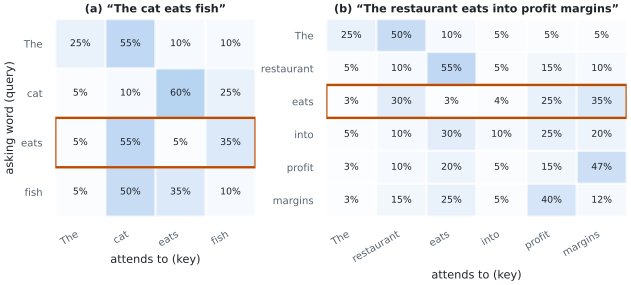
The word “eats” ends up with a completely different representation in each sentence because it attends to different words. That is the whole trick: one word, many possible meanings, and attention picking the right neighbors to define it.
Behind the listening there is arithmetic. The standard analogy — and the one this paper sticks to — is a library, shown in Figure 15.

Each word is transformed into three versions of itself:
Query (Q): the visitor’s question — “what information do I need?”
Key (K): the catalog card — “what information do I offer?”
Value (V): the book’s content — “here is my actual information.”
Crucially, every word plays all three roles at once: it asks (Q), it advertises (K), it delivers (V). One visit to the library, with every book simultaneously a visitor and a shelf.
The librarian compares the question with every card. Questions similar to a card get a high compatibility score; the score is computed by multiplying the query by the key (a dot product). For our “eats” query: \(\mathrm{s}(\text{eats} \rightarrow \text{cat}) = 3.40\), \(\mathrm{s}(\text{eats} \rightarrow \text{fish}) = 2.95\), \(\mathrm{s}(\text{eats} \rightarrow \text{The}) = 1.00\). Figure 16 places the four steps in one pipeline.

Raw scores are just numbers; attention is a budget. A
function called softmax converts the scores into
percentages that always sum to 100%: the “eats” query turns the scores
above into 5% / 55% / 5% / 35% over “The / cat / eats /
fish”. Figure 17 shows the conversion. High
compatibility means “focus attention here”; low compatibility means
“ignore this” — back in the noisy room, the voice you decided to filter
out.
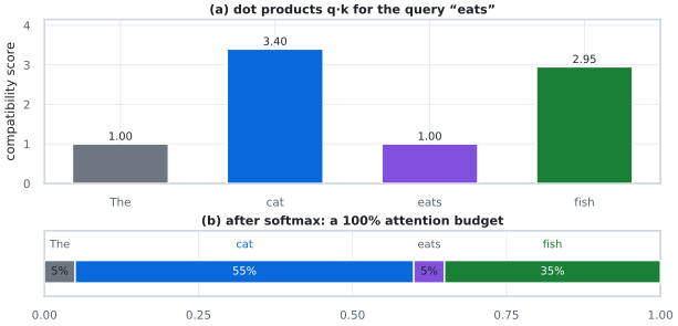
softmax, the same four
numbers become an attention budget that sums to exactly
100%.Finally the visitor leaves the library with a weighted mix of contents. If “eats” places 55% of its budget on “cat” and 35% on “fish”, then 55% of cat’s value and 35% of fish’s value are blended into the new representation of “eats”: \[\text{new ``eats''} \;=\; 5\%\cdot v_{\text{The}} + 55\%\cdot v_{\text{cat}} + 5\%\cdot v_{\text{eats}} + 35\%\cdot v_{\text{fish}}. \label{eq:tut-mix}\] That blended vector is what the rest of the network sees: a representation of “eats” that already contains who eats and what gets eaten.
Transformers never run one attention but many heads in parallel — as if the sentence were analyzed by a team of specialists, each asking a different question about it (Figure 18):
Analyst 1 (grammar): “who does it?” — links cat \(\rightarrow\) eats.
Analyst 2 (object): “what receives it?” — links eats \(\rightarrow\) fish.
Analyst 3 (time): “when / how often?” — tracks verb tense and time words.
Analyst 4 (style): “which articles and modifiers?” — tracks “the”, “a”, adjectives.

Each head learns its own focus pattern from data, and their reports are concatenated and re-mixed by one learned projection. Together they capture far more than any single head could — grammar, roles, time and style at once.
One attention step still sees shallow patterns, so transformers stack the same block many times (12 to 48 in practical models). The analogy: editing an essay in successive passes (Figure 19).
First pass — fix spelling and basic grammar: recognize words, forms, gender.
Second pass — improve clarity of each sentence: who does what to whom.
Third pass — ensure consistency and narrative flow: idioms, relations, abstract meaning.

Each layer re-reads what the previous layer produced and refines it: early layers capture basic features, later layers understand complex relations and abstract concepts. No layer is told what to look for — the passes organize themselves during training.
The attention mechanism was revolutionary because:
Parallelism: any word can be compared with any other word at once (no sequential processing, unlike earlier recurrent systems) — fast on modern hardware.
Flexibility: the patterns are learned from data; nobody programs the rules.
Scalability: the same mechanism works from a sentence to millions of words of context.
Generality: translation, summarization, question answering, generation, computer vision, audio — one mechanism, many tasks.
Dense attention buys its power by comparing every word with every other word, and that price grows fast.
A 1,000-word document forces \(1{,}000 \times 1{,}000 = 1{,}000{,}000\) word-to-word comparisons, and the cost squares as the document grows. Figure 20 shows the growth against the friendlier alternatives discussed below.
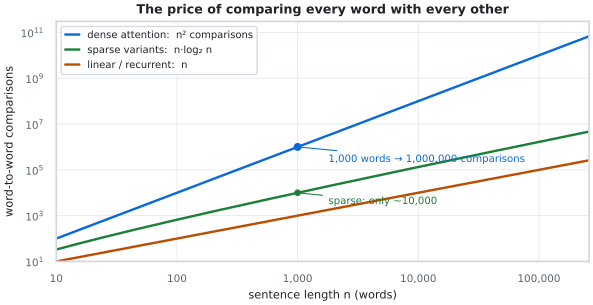
During inference (using a trained model), the keys and values of every past word must be stored — the library keeps every book on the table just in case a later query needs it. For long contexts this cache dominates GPU memory.
Transformers were designed for powerful TPUs and GPUs; running them on phones or embedded devices is challenging.
The rest of this paper is a catalog of ways to keep the benefits of attention while paying less. Each keeps our analogies:
Sparse attention: stop browsing every card in the library — visit only nearby shelves and a few strategic ones. Complexity drops from \(\mathcal{O}(n^2)\) to \(\mathcal{O}(n \log n)\) or \(\mathcal{O}(n)\).
Recurrent models (e.g. Mamba): take notes as you read, instead of re-listening to the whole room for every new word — an old idea (recurrence) rebuilt with modern efficiency.
Gated attention: a gatekeeper decides which of your notes are worth keeping and which to fade out, so less needs to be stored.
Quantization: write each number with fewer digits (small integers instead of wide decimals), shrinking memory with minimal loss of precision.
These innovations are exactly what this toolkit (Frankenstein) lets you experiment with, and the annexes that follow are guided tours of each family.
A transformer is a network that contextualizes: it re-reads every word in the light of all its neighbors (the ambiguous “bank”).
Attention is selective listening: each word focuses its limited 100% budget on the neighbors that define it (the noisy room).
The arithmetic is a library visit: query asks,
key advertises, value delivers; dot
products score compatibility, softmax turns scores into a
100% budget, and the values are mixed by that budget.
Multiple heads are a team of analysts with one question each; stacked layers are successive editing passes, each refining the last.
The catch: dense attention compares everyone with everyone — \(\mathcal{O}(n^2)\) — which is why sparse, recurrent, gated and quantized variants exist.
Every later annex of this paper is a deeper tour of one of those variants; the analogies of Table 2 will keep coming back.
This annex synthesizes the dense, recurrent, and memory-augmented transformer families. The field has evolved toward several primary paradigms: dense global attention with variants, key-value head compression via grouped-query attention, recurrent state compression with decay, selective state-space models, continuous-depth numerical integration, token-indexed value memory, and memory-augmented architectures. Understanding this taxonomy illuminates fundamental tradeoffs between expressiveness, computational cost, memory footprint, and deployment simplicity.

Standard multi-head self-attention computes scaled dot-product similarity between token embeddings:
Input: Query matrix \(\mathbf{Q} \in \mathbb{R}^{n \times d}\), Key matrix \(\mathbf{K} \in \mathbb{R}^{n \times d}\), Value matrix \(\mathbf{V} \in \mathbb{R}^{n \times d}\) \(\text{scores} \gets \frac{\mathbf{Q}\mathbf{K}^\top}{\sqrt{d}} \in \mathbb{R}^{n \times n}\) \(\text{attention\_\allowbreak weights} \gets \texttt{softmax}(\text{scores}, \text{axis}=1) \in \mathbb{R}^{n \times n}\) Output: \(\mathbf{Y} = \text{attention\_\allowbreak weights} \cdot \mathbf{V} \in \mathbb{R}^{n \times d}\)
For autoregressive generation, KV caching stores past keys and values to avoid \(\mathcal{O}(n^2)\) recomputation. However, this linearly growing cache occupies \(\sim n \cdot d_{\text{hidden}}\) bytes, which can consume hundreds of gigabytes for billion-parameter models. Standard attention achieves perfect expressiveness within the context window—any token can attend to any other token with learned weights—but pays the price of dense computation.
Training complexity: \(\mathcal{O}(n^2 \cdot d)\) time, \(\mathcal{O}(n^2)\) space (attention matrix materialization).
Inference complexity: \(\mathcal{O}(n)\) time per token, \(\mathcal{O}(n)\) space (KV cache).
Strengths: Unparalleled expressiveness; perfect history recall; highly parallelizable.
Weaknesses: Quadratic bottleneck prohibits very long contexts; KV cache dominates memory during generation.

Sigmoid attention replaces row-wise softmax with element-wise sigmoid activation :
Input: \(\mathbf{Q}, \mathbf{K}, \mathbf{V}\) as above, learnable bias \(\mathbf{b} \in \mathbb{R}^{n \times n}\) \(\text{logits} \gets \frac{\mathbf{Q}\mathbf{K}^\top}{\sqrt{d}} + \mathbf{b}\) \(\text{attention\_\allowbreak weights} \gets \sigma(\text{logits})\) Output: \(\mathbf{Y} = \text{attention\_\allowbreak weights} \odot \mathbf{V}\)
Unlike softmax, sigmoid does not enforce a probability distribution (weights need not sum to 1), enabling stronger token independence. Theoretical analysis via mixture-of-experts shows sigmoid achieves superior sample complexity: \(\mathcal{O}(n^{-0.51})\) convergence for ReLU experts versus softmax’s \(\mathcal{O}(n^{-0.24})\). However, empirical training revealed gradient instabilities at scale. The remedy is hybrid-norm—adding normalization after the attention output—which stabilizes gradients without sacrificing the theoretical benefits of element-wise gating.
Training complexity: \(\mathcal{O}(n^2 \cdot d)\) (identical to standard), but element-wise operations enable 17% inference speedup via FlashSigmoid.
Inference complexity: \(\mathcal{O}(n)\) per token with KV cache (asymptotically same, but lower constant factors).
Strengths: Overcomes zero-sum competition; avoids row-wise synchronization; hardware-friendly implementation.
Weaknesses: Requires careful stabilization (hybrid-norm); training instability at large scales without auxiliary loss.

Grouped-query attention bridges multi-head attention (MHA) and multi-query attention (MQA) by partitioning query heads into groups, each sharing a single key-value head. If \(h\) is the total number of attention heads, \(h_k\) is the number of key-value heads, and \(G = h / h_k\) is the group size, then every group of \(G\) query heads shares one KV head:
Input: \(\mathbf{Q} \in \mathbb{R}^{n \times h \cdot d_h}\), \(\mathbf{K} \in \mathbb{R}^{n \times h_k \cdot d_h}\), \(\mathbf{V} \in \mathbb{R}^{n \times h_k \cdot d_h}\) \(\mathbf{K}_{\text{full}} \gets \texttt{repeat\_\allowbreak interleave}(\mathbf{K}, G)\) \(\mathbf{V}_{\text{full}} \gets \texttt{repeat\_\allowbreak interleave}(\mathbf{V}, G)\) \(\text{scores} \gets \frac{\mathbf{Q}\mathbf{K}_{\text{full}}^\top}{\sqrt{d_h}} \in \mathbb{R}^{n \times n}\) \(\text{attention\_\allowbreak weights} \gets \texttt{softmax}(\text{scores}, \text{axis}=1)\) Output: \(\mathbf{Y} = \text{attention\_\allowbreak weights} \cdot \mathbf{V}_{\text{full}} \in \mathbb{R}^{n \times h \cdot d_h}\)
GQA interpolates smoothly between MHA (\(h_k = h\), \(G = 1\)) and MQA (\(h_k = 1\), \(G = h\)). The key advantage is a tunable tradeoff between KV-cache footprint and representational capacity. Each additional KV head consumes \(2 \cdot d_h \cdot n\) extra bytes in the cache, so reducing \(h_k\) yields proportional memory savings.
Training complexity: \(\mathcal{O}(n^2 \cdot h \cdot d_h)\) (identical to MHA after head expansion).
Inference complexity: \(\mathcal{O}(n)\) per token, \(\mathcal{O}(h_k \cdot n \cdot d_h)\) KV-cache space.
Strengths: Flexible head-count tradeoff; proven at scale (Llama 2 & 3 use \(h_k = 8\) KV heads with \(h = 32\) query heads); reduces KV-cache by \(G \times\); supports fast inference with FlashAttention.
Weaknesses: Fewer KV heads can reduce representational capacity in small models; requiring \(h_k\) to divide \(h\) constrains architectural choices.

Continuum Attention replaces discrete softmax retrieval with exact integration over a continuous, piecewise-linear memory trajectory. Adjacent keys and values are interpolated so that \(\mathbf{k}(t)\) and \(\mathbf{v}(t)\) are defined at every position of the visible domain: \[\mathbf{k}_j(u) = (1-u)\,\mathbf{k}_{j-1} + u\,\mathbf{k}_j, \qquad \mathbf{v}_j(u) = (1-u)\,\mathbf{v}_{j-1} + u\,\mathbf{v}_j,\] with \(u = t-(j-1)\in[0,1]\) on the interval \([j-1,j]\); constant half-token extensions cover \([-1/2,0]\) and \([i,i+1/2]\). Each query induces an exponential relevance density over the visible prefix, \[s_i(t) = \frac{\gamma}{\sqrt{d_h}}\,\mathbf{q}_i^\top \mathbf{k}(t), \qquad p_i(t) = \frac{\exp(s_i(t))}{Z_i}, \qquad \mathbf{o}_i = \int_{-1/2}^{i+1/2} p_i(t)\,\mathbf{v}(t)\,dt,\] where \(\gamma>0\) is the score gain (\(\gamma=1/\tau\)). Since the key trajectory is linear within a segment, the score is affine, \(s_{ij}(u) = a_{ij} + u\,\Delta_{ij}\) with \(a_{ij}=s_i(j-1)\), \(b_{ij}=s_i(j)\) and \(\Delta_{ij}=b_{ij}-a_{ij}\), so the integrals have closed forms in the exponential moments \(J_n(\Delta)=\int_0^1 u^n e^{\Delta u}\,du\): \[\begin{aligned} J_0(\Delta) &= \frac{e^{\Delta}-1}{\Delta}, \qquad J_1(\Delta) = \frac{(\Delta-1)e^{\Delta}+1}{\Delta^2}, \\ M_{ij} &= e^{a_{ij}} J_0(\Delta_{ij}), \qquad \mathbf{U}_{ij} = e^{a_{ij}}\big[(J_0-J_1)\,\mathbf{v}_{j-1} + J_1\,\mathbf{v}_j\big], \\ Z_i &= \tfrac12 e^{s_i(0)} + \tfrac12 e^{s_i(i)} + \sum_{j=1}^{i} M_{ij}, \qquad \mathbf{o}_i = \frac{\mathbf{U}_i^{\mathrm{cap}} + \sum_{j=1}^{i}\mathbf{U}_{ij}}{Z_i}, \end{aligned}\] with \(\mu(\Delta)=J_1/J_0\) the normalized retrieval position inside a segment. Because the contributions are nonnegative, CA is equivalently a normalized nonnegative weighted sum of the original values, \(\mathbf{o}_i = \sum_{j\le i} w_{ij}\mathbf{v}_j\) with \(w_{ij}\ge 0\) and \(\sum_j w_{ij}=1\); equal visible scores reduce exactly to uniform causal attention and \(o_0=v_0\). The learned-gain variant adds one scalar per head (\(\gamma=\exp(\rho)\), initialized at \(\gamma=1\) in the 101M model; the fixed CA-P variant uses \(\gamma=1/0.30\) and adds no parameters). The encoder (bidirectional) form integrates over the full trajectory \([-1/2,n-1/2]\) – the natural symmetric extension of the causal-only paper.
Input: \(\mathbf{Q}, \mathbf{K}, \mathbf{V} \in \mathbb{R}^{n \times d_h}\), gain \(\gamma>0\) \(\mathbf{S} \gets \gamma\,\mathbf{Q}\mathbf{K}^\top/\sqrt{d_h}\) mask \(\mathbf{S}\) to the visible prefix; subtract the row maximum \(m\) (stability) \(\Delta_{ij} \gets \mathbf{S}_{j}-\mathbf{S}_{j-1}\); \(J_0,J_1 \gets\) Eqs. (11)–(12) (series near \(\Delta=0\)) \(M_{ij} \gets e^{a_{ij}-m}J_0\), \(w^{(L)}_{ij}\gets M_{ij}(1-\mu)\), \(w^{(R)}_{ij}\gets M_{ij}\mu\) add the half-token caps \(\tfrac12 e^{s_i(0)-m}\) and \(\tfrac12 e^{s_i(i)-m}\); normalize by \(Z_i\) Output: \(\mathbf{o}_i = \sum_{j\le i} w_{ij}\mathbf{v}_j\)
Training complexity: \(\mathcal{O}(n^2 d)\) – identical to dense softmax; the closed-form moments replace the softmax (no quadrature).
Inference complexity: \(\mathcal{O}(n)\) per token with a KV cache; the effective weights are recomputed row-locally over the cached prefix each step (exact).
Strengths: Exact continuous retrieval with normalized nonnegative effective weights; zero parameters beyond the projections in the fixed-gain form; strong multilingual and zero-shot results (FLORES macro 1.8915 BPB, a 5.8% reduction versus the strongest baseline and the best score in every language; HellaSwag and ARC-Challenge best among the baselines); 42% fewer training bytes to a matched 1.10 BPB threshold than a matched Transformer.
Weaknesses: The quadratic attention arithmetic persists; source-code performance is the weakest of the five architectures (Stack-smol 3.3451 BPB); reduced robustness to byte deletion and “antspeak” perturbations.

Exclusive Self Attention starts from the observation that in trained Transformers the attention output \(\mathbf{y}_i\) keeps a large cosine similarity with the token’s own value vector \(\mathbf{v}_i\)—the attention similarity bias—and that this similarity grows with depth. Since the residual path and the following FFN already carry the point-wise information of position \(i\), that component is redundant and competes with the layer’s actual job, context modeling. XSA therefore subtracts it explicitly. The first line is standard causal softmax attention: \[\mathbf{q}_i = \mathbf{W}_q\mathbf{x}_i, \quad \mathbf{k}_j = \mathbf{W}_k\mathbf{x}_j, \quad \mathbf{v}_j = \mathbf{W}_v\mathbf{x}_j, \quad a_{i,j} = \frac{\exp(\mathbf{q}_i^\top\mathbf{k}_j)}{\sum_{j'=1}^{i}\exp(\mathbf{q}_i^\top\mathbf{k}_{j'})}, \quad \mathbf{y}_i = \sum_{j=1}^{i} a_{i,j}\mathbf{v}_j,\] and the exclusive step projects the output orthogonally out of the self value direction: \[\hat{\mathbf{v}}_i = \frac{\mathbf{v}_i}{\|\mathbf{v}_i\|_2}, \qquad \mathbf{z}_i = \mathbf{y}_i - \big(\mathbf{y}_i^\top \hat{\mathbf{v}}_i\big)\,\hat{\mathbf{v}}_i .\] The step is parameter-free, row-local (it only consumes the current token’s value) and differentiable, so it trains end-to-end with the usual four projections \(\mathbf{W}_q,\mathbf{W}_k,\mathbf{W}_v,\mathbf{W}_o \in \mathbb{R}^{H\times H}\); the parameter count is exactly \(4H^2\), identical to standard attention. Removing the self direction can be read as an implicit attention sink: undesired mass is parked on the diagonal \(a_{i,i}\) and then discarded, which is consistent with the observed robustness to explicit sink tokens.
Input: \(\mathbf{x}\); \(\mathbf{W}_q,\mathbf{W}_k,\mathbf{W}_v,\mathbf{W}_o\); \(n_h\) heads of width \(d_h\) \(\mathbf{Q}\gets\mathbf{x}\mathbf{W}_q\), \(\mathbf{K}\gets\mathbf{x}\mathbf{W}_k\), \(\mathbf{V}\gets\mathbf{x}\mathbf{W}_v\) \(\mathbf{Y} \gets \texttt{softmax}(\mathbf{Q}\mathbf{K}^\top/\sqrt{d_h} + \text{causal mask})\,\mathbf{V}\) \(\hat{\mathbf{V}} \gets \mathbf{V} / \|\mathbf{V}\|_2\) \(\mathbf{Z} \gets \mathbf{Y} - (\mathbf{Y}\odot\hat{\mathbf{V}})\text{-sum}_{d_h}\cdot\hat{\mathbf{V}}\) Output: \(\mathbf{Z}\mathbf{W}_o\)
Training complexity: \(\mathcal{O}(n^2 d)\) – the softmax attention dominates; the exclusion is \(\mathcal{O}(nd)\) and measured as minimal overhead (speed and memory curves overlap the baseline across sequence lengths and model widths).
Inference complexity: \(\mathcal{O}(n)\) per token with a plain KV cache; the exclusion reads only the newly computed \(\mathbf{v}_i\), so incremental decoding is exact (class (i)).
Strengths: Zero additional parameters; two-line change; consistent training/validation gains at 0.7B, 1.3B and 2.7B parameters on FineWeb-100BT (+0.26, +1.03 and +1.36 average downstream points over SA); the margin grows with sequence length (512 to 16k) and is stable across learning rates and attention-sink configurations.
Weaknesses: Evidence is language-modeling only; the paper offers no theoretical grounding beyond the empirical motivation; per-token L2 normalization is an extra (small) kernel compared with vanilla SDPA; the encoder (bidirectional) variant used by this toolkit is a mask-agnostic extension of the paper’s causal formulation.

Multi-Token Attention targets the single-token bottleneck of soft attention: every weight \(a_{ij}\) is decided by one query and one key vector, so a context region identified by several tokens (a sentence mentioning both “Alice” and “rabbit”) must be compressed into a single vector. MTA keeps the quadratic attention skeleton and makes neighbouring queries, keys and heads interact through small learned convolutions over the score map. The key-query convolution mixes the logits of a window of \(c_q\) queries and \(c_k\) keys, per head: \[a_{ij} = \operatorname{Softmax}\Big(\sum_{i'=0}^{c_q-1}\ \sum_{j'=-\lfloor c_k/2\rfloor}^{\lceil c_k/2\rceil-1} \mathbf{1}_{i\ge j-j'}\ \theta_{i',j'}\ \mathbf{q}_{i-i'}\mathbf{k}_{j-j'}^{\top}/\sqrt{d_h}\Big), \label{eq:mta-exact}\] and, because that indicator would require bespoke CUDA kernels, the default implementation applies the existing causal mask twice: \[\mathbf{A} = \operatorname{Softmax}\Big(\operatorname{Mask}_{-\infty}\big(\operatorname{Conv2d}_{\theta}(\operatorname{Mask}_{0}(\hat{\mathbf{A}}))\big)\Big), \qquad \mathbf{A} = \operatorname{Mask}_{0}\Big(\operatorname{Conv2d}_{\theta}\big(\operatorname{Softmax}(\operatorname{Mask}_{-\infty}(\hat{\mathbf{A}}))\big)\Big), \label{eq:mta-pre}\] where the first expression is the pre-softmax variant (the paper’s default) and the second the post-softmax variant (additive rather than multiplicative interaction); both are applied by default. Head mixing partitions the \(n_h\) heads into \(n_h/c_h\) non-overlapping groups and mixes each group with its own \(c_h\times c_h\) kernel, \[\mathbf{A}^{1}_{\text{new}} = w_{11}\mathbf{A}^{1}+w_{12}\mathbf{A}^{2}, \qquad \mathbf{A}^{2}_{\text{new}} = w_{21}\mathbf{A}^{1}+w_{22}\mathbf{A}^{2}, \label{eq:mta-head}\] so attention maps can be combined across heads (a post-softmax \(2\times2\) mixing is equivalent to doubling the rank of the value/output projections, Appendix B of the paper). Finally a grouped normalization over each set of \(c_h\) heads followed by a per-head sigmoid gate, \(\operatorname{diag}(\sigma(\mathbf{g}))\operatorname{GroupNorm}(\mathbf{A}\mathbf{V})\), pushes back against the residual stream and lets the model switch heads on and off across layers; the paper reports 10.90 validation perplexity with scalar gating versus 11.03 without scaling and 11.41 with layer-norm scaling. Kernels are identity-initialized (the best-converging choice) and the mixer adds only about \(0.001\%\) of the parameters at 880M scale: \(n_h(2c_qc_k + c_h) + 2H + n_h\), i.e. one scalar per head for the gate, an affine group norm, and the kernels.
Input: \(\mathbf{x}\); \(\mathbf{W}_q,\mathbf{W}_k,\mathbf{W}_v,\mathbf{W}_o\); knobs \(c_q,c_k,c_h\) \(\mathbf{Q}\gets\mathbf{x}\mathbf{W}_q\), \(\mathbf{K}\gets\mathbf{x}\mathbf{W}_k\), \(\mathbf{V}\gets\mathbf{x}\mathbf{W}_v\); \(\hat{\mathbf{A}}\gets\mathbf{Q}\mathbf{K}^\top/\sqrt{d_h}\) \(\hat{\mathbf{A}}\gets\operatorname{Mask}_{0}(\hat{\mathbf{A}})\); \(\hat{\mathbf{A}}\gets\operatorname{Conv2d}_{\theta_{\text{pre}}}(\hat{\mathbf{A}})\) \(\mathbf{A}\gets\operatorname{Softmax}(\operatorname{Mask}_{-\infty}(\hat{\mathbf{A}}))\) \(\mathbf{A}\gets\) head conv \(w\) over groups of \(c_h\); \(\mathbf{A}\gets\operatorname{Mask}_{0}(\operatorname{Conv2d}_{\theta_{\text{post}}}(\mathbf{A}))\) \(\mathbf{O}\gets\operatorname{diag}(\sigma(\mathbf{g}))\operatorname{GroupNorm}(\mathbf{A}\mathbf{V})\) Output: \(\mathbf{O}\mathbf{W}_o\)
Training complexity: \(\mathcal{O}(n^2 d_h n_h + n^2 c_q c_k n_h)\) – still quadratic in the sequence length, with a small constant from the kernels; the score map must be materialised, so fused SDPA kernels are not compatible (the paper’s stated limitation).
Inference complexity: \(\mathcal{O}(n d_h n_h)\) per step with a KV cache plus an \(\mathcal{O}(c_q c_k n_h)\) convolution correction; decode keeps the classic KV cache and a FIFO tail of the last \(c_q-1\) queries, so the double-masked convolution is reproduced exactly (classes (i)+(v)).
Strengths: Consistent gains at 880M/105B SlimPajama tokens over Transformer, Diff Transformer and Talking-Heads baselines (average validation perplexity 10.91 versus 11.25, 11.15 and 11.04; 44.9 versus 43.7 average zero-shot points), large long-context retrieval gains (multi-needle, BabiLong, LAMBADA) with \(+0.001\%\) parameters, and near-identity kernels that are learned to be diagonal “sentence-matching”, priming or edge-detecting filters.
Weaknesses: Incompatible with optimized attention kernels (the score map is materialised); the key-query convolution is applied on every fourth layer in the reference run for efficiency, so the full-per-layer variant costs more arithmetic than reported; the encoder (bidirectional) form used by this toolkit drops both causal masks, an extension of the paper’s causal-only formulation.
The memory family groups Titans (the attention window implemented here), Engram (Appendix 24) and Memory Attention; this annex covers the attention-side members.

Memory Attention removes the dedicated value projection and constructs values from contextual keys plus layer-specific token memory. With token IDs \(s\), vocabulary size \(N\) and \(d_v = H_{KV} d_h\):
Input: hidden states \(X \in \mathbb{R}^{T \times d}\), token IDs \(s\), table \(E \in \mathbb{R}^{N \times d_v}\) \(M \gets \mathrm{Norm}(E[s]) \in \mathbb{R}^{T \times d_v}\) \(Q \gets X W_Q\), \(K \gets X W_K\), \(V \gets K + M\) \(Q_R \gets \mathrm{RoPE}(Q)\), \(K_R \gets \mathrm{RoPE}(K)\) Output: \(Y = \mathrm{softmax}\!\left(\tfrac{Q_R K_R^\top}{\sqrt{d_k}} + C\right) V\)
The output decomposes as \(O_{\mathrm{MA}} = A(K{+}M) = AK + AM\): a contextual retrieval term over keys and a memory retrieval term aggregated under the same attention distribution. Across \(L\) replaced layers, MA swaps the standard \(L\,d\,d_v\) value-projection parameters for \(L(N d_v + p_{\mathrm{norm}})\) memory and normalization parameters — added capacity accessed by lookup instead of dense computation. At inference the per-row normalization is folded into the table (\(E[i] \gets \mathrm{Norm}(E[i])\)), reducing online value construction to lookup and addition while retaining a conventional KV cache. The paper reports improved LAMBADA/WikiText perplexity and average downstream accuracy across MHA/GQA/MQA backbones at matched token budgets, with \(1.42\times\)/\(1.16\times\) token efficiency; the comparison includes the additional memory parameters, so it does not isolate structure from capacity. MA-Offload (CPU-resident tables with prefetching) and MA-Recall (reconstructing historical values as \(V_{1:T} = K_{1:T} + E[s_{1:T}]\) for a \({\sim}50\%\) smaller value cache) are analyzed but not implemented here.
Training complexity: \(\mathcal{O}(n^2 d)\) attention with \(\mathcal{O}(n d_v)\) lookup+norm+add value construction (replacing the \(\mathcal{O}(n\, d\, d_v)\) projection).
Inference complexity: \(\mathcal{O}(n)\) per token with a conventional KV cache; \(N d_v\) extra parameters per layer.
Strengths: Extra capacity without dense-compute growth; layer-specific token representations; exact standard-attention aggregation; KV-cache-compatible by construction.
Weaknesses: Parameter count grows with the vocabulary (\(N \gg d\)); needs token IDs (text-only); the reported gains are not parameter-matched.

RetNet unifies three computation paradigms: parallel training, recurrent inference, and chunkwise deployment. Its core innovation is the retention mechanism, which uses a fixed exponential decay matrix to model temporal importance:
Parallel (training) form: \(\text{decay\_\allowbreak matrix}[i,j] \gets \gamma^{i-j}\) for \(i \geq j\), else \(0\) \(\text{decay\_\allowbreak matrix}[i,j] \gets 0\) for \(i < j\) \(\mathbf{Y}_{\text{parallel}} \gets (\mathbf{Q}\mathbf{K}^\top \odot \text{decay\_\allowbreak matrix}) \mathbf{V}\)
Recurrent (inference) form: \(\mathbf{s}_t \gets \gamma \mathbf{s}_{t-1} + \mathbf{k}_t \mathbf{v}_t^\top\) \(\mathbf{y}_t \gets \mathbf{q}_t \mathbf{s}_t\)
The decay scalar \(\gamma \in (0,1)\) controls the temporal window. RetNet uses multi-scale retention with different \(\gamma\) values per head (e.g., \(\gamma = 1 - 2^{-5}, 1 - 2^{-6}, \ldots\)), allowing short-term and long-term dependencies simultaneously. Chunkwise recurrent mode divides sequences into chunks, processes each chunk in parallel, and threads a recurrent state between chunks.
Training complexity: \(\mathcal{O}(n^2 \cdot d)\) (parallel), or \(\mathcal{O}(n \cdot c \cdot d)\) (chunkwise recurrent with chunk size \(c\)).
Inference complexity: \(\mathcal{O}(1)\) per token, \(\mathcal{O}(d^2)\) state space (fixed matrix).
Strengths: Constant-time inference; triple computation paradigm; multi-scale consolidation.
Weaknesses: Fixed decay imposes rigid inductive bias; may truncate learned long-range patterns.

Mamba frames recurrence as a continuous-time dynamical system with input-dependent parameters, achieving both linear training and constant-time inference:
Continuous dynamics: \(h'(t) = \mathbf{A} h(t) + \mathbf{B} x(t)\), \(y(t) = \mathbf{C} h(t)\) Discretization with step size \(\Delta_t\): \(\bar{\mathbf{A}}_t \gets \exp(\Delta_t \mathbf{A})\) \(\bar{\mathbf{B}}_t \gets (\Delta_t \mathbf{A})^{-1} (\exp(\Delta_t \mathbf{A}) - \mathbf{I}) \Delta_t \mathbf{B}_t\) Recurrent update: \(\Delta_t \gets \text{softplus}(\text{Linear}(x_t))\) \(\mathbf{B}_t \gets \text{Linear}(x_t)\), \(\mathbf{C}_t \gets \text{Linear}(x_t)\) \(h_t \gets \bar{\mathbf{A}}_t h_{t-1} + \bar{\mathbf{B}}_t x_t\) \(y_t \gets \mathbf{C}_t h_t\)
The critical innovation is that \(\mathbf{A}\) (the system matrix) is not input-dependent, but \(\Delta_t\), \(\mathbf{B}_t\), and \(\mathbf{C}_t\) are, making the system time-varying. This selectivity allows the model to ignore irrelevant information by setting \(\Delta_t\) near zero, effectively creating a gate. A hardware-aware parallel scan algorithm implements the recurrence efficiently on GPUs by fusing computation within SRAM, avoiding expensive HBM bandwidth.
Training complexity: \(\mathcal{O}(n \cdot d)\) via hardware-aware scan (linear in sequence length).
Inference complexity: \(\mathcal{O}(1)\) per token, \(\mathcal{O}(d)\) state (hidden vector).
Strengths: Achieves linear training and constant-inference simultaneously; practical on long sequences (millions of tokens).
Weaknesses: State vector compression can weaken exact copying and dense associative recall versus full attention.

The ODE Transformer interprets network depth as numerical integration of a continuous dynamical system, using higher-order Runge-Kutta solvers to reduce truncation error:
Continuous formulation: \(\frac{dh(t)}{dt} = f_\theta(h(t), t)\) where \(f_\theta\) is the transformer sub-network Runge-Kutta-4 discrete approximation: \(k_1 \gets f_\theta(h_t, t)\) \(k_2 \gets f_\theta(h_t + \tfrac{1}{2}k_1, t + \tfrac{1}{2}\Delta t)\) \(k_3 \gets f_\theta(h_t + \tfrac{1}{2}k_2, t + \tfrac{1}{2}\Delta t)\) \(k_4 \gets f_\theta(h_t + k_3, t + \Delta t)\) \(h_{t+1} \gets h_t + \frac{\Delta t}{6}(k_1 + 2k_2 + 2k_3 + k_4)\)
Instead of simple Euler residual connections \(h_{t+1} = h_t + f_\theta(h_t)\), the RK4 block computes four intermediate evaluations and combines them with classical RK4 weights. To avoid vanishing gradients, the architecture introduces learned gating that interpolates between intermediate approximations:
\(g \gets \sigma(\text{Linear}([k_1, k_2, k_3, k_4]))\) \(h_{t+1} \gets h_t + g \cdot k_1 + (1-g) \cdot k_2\)
This formulation reduces the effective number of parameters through weight sharing—the same \(f_\theta\) is evaluated multiple times—while providing richer trajectory refinement.
Training complexity: \(\mathcal{O}(k \cdot n^2 \cdot d)\) where \(k\) is the RK order (4 for RK4).
Inference complexity: \(\mathcal{O}(k \cdot n)\) per token (higher constant overhead).
Strengths: Significantly higher accuracy on generation tasks (state-of-the-art BLEU); parameter-efficient via weight sharing.
Weaknesses: High per-step compute; inference latency increases by constant factor \(k\); complex gating required for stability.

The Titans architecture introduces an orthogonal dimension: instead of static weights, the model maintains a learnable memory that is updated during inference based on a surprise-driven signal:
Local short-term attention: Apply standard or sparse attention within a fixed context window \(c\) \(y_t^{\text{local}} \gets \text{Attention}(q_t, k_{[t-c:t]}, v_{[t-c:t]})\) Memory update signal (surprise): \(S_t \gets \eta_t S_{t-1} - \theta_t \nabla_\ell(\mathcal{M}_{t-1}; x_t)\) \(\mathcal{M}_t \gets (1 - \alpha_t) \mathcal{M}_{t-1} + S_t\) Long-term memory retrieval: \(y_t^{\text{memory}} \gets \mathcal{M}_t^* (q_t)\) Output combination: \(y_t \gets y_t^{\text{local}} + \text{gate}(y_t^{\text{memory}})\)
The memory module \(\mathcal{M}\) is literally updated during the forward pass by computing gradients of an associative loss and applying SGD steps with momentum. The decay rates \(\eta_t, \theta_t, \alpha_t\) are themselves input-dependent, allowing the model to switch memory paradigms when context shifts.
Training complexity: Roughly \(\mathcal{O}(c^2 + n \cdot f)\) where \(c\) is local window and \(f\) is memory update overhead.
Inference complexity: \(\mathcal{O}(c^2)\) local attention plus \(\mathcal{O}(1)\) memory retrieval per token.
Strengths: Handles extreme context lengths; enables true associative recall; memory adapts to input.
Weaknesses: Significantly more complex; inference includes gradient computation; higher coordination overhead.
The codebase selects a mixer per block from the configured
layer_pattern. The dispatch logic routes inference-time
sparse blocks (fasa, sparge) to standard dense
attention while the model is in training mode, and to their sparse
implementation during evaluation; all other blocks route to the
corresponding family implementation.
Hidden states \(H\), pattern \(P\), layer index \(\ell\) \(m \gets P[\ell \bmod |P|]\) \(H \gets \text{softmax-attention}(H)\) \(H \gets \text{softmax-attention}(H)\) \(H \gets \text{sigmoid-attention}(H)\) \(H \gets \text{continuum-attention}(H)\) \(H \gets \text{multi-token-attention}(H)\) \(H \gets \text{memory-attention}(H)\) \(H \gets \text{retention}(H)\) \(H \gets \text{selective-ssm}(H)\) \(H \gets \text{rk-step}(H)\) \(H \gets \text{sparse-attention-family}(H)\) \(H \gets \text{gated-attention-family}(H)\) \(H \gets \text{memory-augmented-attn}(H)\) \(H\)
The field exhibits a clear progression along two axes: (i) computational efficiency, moving from \(O(n^2)\) to \(O(n)\) or \(O(1)\), and (ii) memory adaptivity, shifting from static weights to dynamic, test-time updated models. Standard attention remains the expressiveness baseline; Mamba and RetNet represent the practical efficiency frontier; Titans introduces an orthogonal innovation axis (test-time learning). The choice of architecture reflects the fundamental engineering constraint: expressiveness versus deployment cost. The latent-attention family, which compresses the KV cache into a low-rank latent, is covered in Appendix 14.
This annex covers the latent / low-rank KV compression family of attention mechanisms. These architectures compress the per-token key–value state into a low-rank latent vector that is the only quantity materialised in the KV cache during decoding, then reconstruct full multi-head keys and values on the fly. The family unifies grouped-query, latent, factorised, and temporal-latent designs under a common low-rank bottleneck.

Multi-Head Latent Attention (MLA) compresses the per-token key–value state into a single low-rank latent vector \(c_{KV}\) of rank \(r_{kv}\), which is the only quantity materialised in the KV cache during decoding. A pair of up-projection matrices reconstructs the full multi-head keys and values on the fly, while RoPE is applied to the decompressed query and key tensors so that positional structure is preserved. The authors show that the Pareto-optimal latent width sits near \(r_{kv} = d_{\text{hidden}} / 2\), at which point MLA halves the KV cache yet matches multi-head attention (MHA) quality on small models.
\[c_{KV} = W_{DKV}\, x \in \mathbb{R}^{r_{kv}}, \qquad k = W_{UK}\, c_{KV}, \qquad v = W_{UV}\, c_{KV}, \qquad q = W_{Q}\, x.\] \[\tilde q = \text{RoPE}(q), \quad \tilde k = \text{RoPE}(k), \qquad \text{attn} = \texttt{softmax}\!\left(\frac{\tilde q\, \tilde k^\top}{\sqrt{d_h}}\right) v.\]
Input: hidden state \(x \in \mathbb{R}^{n \times d}\), rank \(r_{kv}\), projections \(W_{DKV}, W_{UK}, W_{UV}, W_{Q}\) \(c_{KV} \gets W_{DKV}\, x\) \(k \gets W_{UK}\, c_{KV}\), \(v \gets W_{UV}\, c_{KV}\) \(q \gets W_{Q}\, x\) \(\tilde q \gets \text{RoPE}(q)\), \(\tilde k \gets \text{RoPE}(k)\) \(\text{weights} \gets \texttt{softmax}(\tilde q\, \tilde k^\top / \sqrt{d_h})\) Output: \(\mathbf{Y} = \text{weights} \cdot v\)
Training complexity: \(\mathcal{O}(n^2 \cdot d)\) (full attention on decompressed heads).
Inference complexity: \(\mathcal{O}(n)\) per token, \(\mathcal{O}(r_{kv} \cdot n)\) KV-cache space (latent only).
Trainable: fully trainable; \(r_{kv}\) is a hyperparameter (Pareto-optimal \(\approx d/2\)).
Strengths: Halves KV cache versus MHA at matched quality; RoPE-compatible; clean latent bottleneck.
Limitations: Up-projection adds decode FLOPs; latent rank is a fixed global budget shared across heads.

Group-Query Latent Attention (GQLA) is a minimal modification of MLA that exposes two algebraically equivalent decoding paths over the same trained weights: an MQA-absorb path (fusing the up-projection into the query, optimal on H100-class hardware) and a GQA-expanded path (materialising full keys/values, optimal on H20 / multi-token-prediction hardware). The two paths are mathematically identical because the up-projection is linear, so \(\texttt{softmax}(q_{\text{absorbed}} \cdot c_{KV}^\top) = \texttt{softmax}((q \cdot W_{UK}^\top) \cdot c_{KV}^\top)\), allowing hardware-adaptive dispatch with no retraining.
Same latent as MLA: \[c_{KV} = W_{DKV}\, x, \qquad k = W_{UK}\, c_{KV}, \qquad v = W_{UV}\, c_{KV}, \qquad q = W_{Q}\, x.\] \[\text{Path A (MQA-absorb): } \text{attn} = \texttt{softmax}\!\left(\frac{(q\, W_{UK}^\top)\, c_{KV}^\top}{\sqrt{d_h}}\right) (W_{UV}\, c_{KV}).\] \[\text{Path B (GQA-expanded): } \text{attn} = \texttt{softmax}\!\left(\frac{q\, k^\top}{\sqrt{d_h}}\right) v, \quad k = W_{UK} c_{KV},\ v = W_{UV} c_{KV}.\]
Input: \(x\), weights \(W_{DKV}, W_{UK}, W_{UV}, W_{Q}\), hardware flag \(\text{hw} \in \{\text{H100}, \text{H20}\}\) \(c_{KV} \gets W_{DKV}\, x\) \(q \gets W_{Q}\, x\) \(q_{\text{abs}} \gets q\, W_{UK}^\top\) \(\text{weights} \gets \texttt{softmax}(q_{\text{abs}}\, c_{KV}^\top / \sqrt{d_h})\) \(\mathbf{Y} \gets \text{weights} \cdot (W_{UV}\, c_{KV})\) \(k \gets W_{UK}\, c_{KV}\), \(v \gets W_{UV}\, c_{KV}\) \(\text{weights} \gets \texttt{softmax}(q\, k^\top / \sqrt{d_h})\) \(\mathbf{Y} \gets \text{weights} \cdot v\) Output: \(\mathbf{Y}\)
Training complexity: \(\mathcal{O}(n^2 \cdot d)\), identical to MLA.
Inference complexity: \(\mathcal{O}(n)\) per token, \(\mathcal{O}(r_{kv} \cdot n)\) latent state; path chosen by hardware.
Trainable: trained once; the two decoding paths reuse the same weights.
Strengths: Hardware-adaptive decode with no quality loss; algebraic equivalence guarantees consistency.
Limitations: Same latent-rank tradeoffs as MLA; path selection is a deployment-time heuristic.

Multi-Head Low-Rank Attention (MLRA) refactors the single MLA latent into \(L\) disjoint sub-heads each of rank \(r/L\), so that the KV cache can be partitioned across \(L\) devices for 4-way tensor-parallel decoding (each device loads only \(1/L\) of the cache). Per-sub-head up-projections reconstruct the corresponding slice of the full heads and are concatenated, yielding a 2.8\(\times\) decode speedup over MLA while preserving the global latent budget.
\[c_{KV} = [c_1, c_2, \ldots, c_L], \quad c_i \in \mathbb{R}^{r/L}, \qquad c_{KV} = W_{DKV}\, x.\] \[k_i = W_{UK}^{(i)}\, c_i, \quad v_i = W_{UV}^{(i)}\, c_i, \qquad k = [k_1; \ldots; k_L], \quad v = [v_1; \ldots; v_L].\] \[\text{attn} = \texttt{softmax}\!\left(\frac{q\, k^\top}{\sqrt{d_h}}\right) v.\]
Input: \(x\), sub-head count \(L\), per-sub-head projections \(W_{UK}^{(i)}, W_{UV}^{(i)}\) \(c_{KV} \gets W_{DKV}\, x = [c_1, \ldots, c_L]\) \(k_i \gets W_{UK}^{(i)}\, c_i\), \(v_i \gets W_{UV}^{(i)}\, c_i\) \(k \gets \texttt{concat}(k_1, \ldots, k_L)\), \(v \gets \texttt{concat}(v_1, \ldots, v_L)\) \(\text{weights} \gets \texttt{softmax}(q\, k^\top / \sqrt{d_h})\) Output: \(\mathbf{Y} = \text{weights} \cdot v\)
Training complexity: \(\mathcal{O}(n^2 \cdot d)\) (full attention on concatenated heads).
Inference complexity: \(\mathcal{O}(n)\) per token, \(\mathcal{O}(r_{kv} \cdot n)\) state partitioned across \(L\) devices.
Trainable: fully trainable; \(L\) controls partition granularity.
Strengths: 2.8\(\times\) decode speedup; clean 4-way tensor-parallel cache sharding; preserves total latent budget.
Limitations: Requires \(L\) to divide \(r_{kv}\); more projection matrices than MLA; inter-device all-reduce on output.

Tucker Attention unifies MHA, GQA and MLA under a single Tucker-style factorisation of the query/key/value weight tensors with independent ranks \(q_{\text{rank}}, k_{\text{rank}}, v_{\text{rank}}\). MHA is recovered when all ranks equal the hidden size, GQA when \(k_{\text{rank}} = v_{\text{rank}} < d\), and MLA when \(k_{\text{rank}} = v_{\text{rank}}\) equals the latent rank. Because the factorisation is a pure linear reparameterisation, the method is fully compatible with FlashAttention and RoPE, and yields an order of magnitude fewer parameters for comparable metrics.
\[\mathbf{Q} = W_{Q,\text{core}}\, W_{Q,\text{factor}}\, x, \qquad \mathbf{K} = W_{K,\text{core}}\, W_{K,\text{factor}}\, x, \qquad \mathbf{V} = W_{V,\text{core}}\, W_{V,\text{factor}}\, x.\] \[\text{attn} = \texttt{softmax}\!\left(\frac{\mathbf{Q}\, \mathbf{K}^\top}{\sqrt{d_h}}\right) \mathbf{V}.\] Special cases: MHA \(\Leftrightarrow q_{\text{rank}} = k_{\text{rank}} = v_{\text{rank}} = d\); GQA \(\Leftrightarrow k_{\text{rank}} = v_{\text{rank}} < d\); MLA \(\Leftrightarrow k_{\text{rank}} = v_{\text{rank}} = r_{kv}\).
Input: \(x\), ranks \(q_{\text{rank}}, k_{\text{rank}}, v_{\text{rank}}\), core/factor matrices \(\mathbf{Q} \gets W_{Q,\text{core}}\, W_{Q,\text{factor}}\, x\) \(\mathbf{K} \gets W_{K,\text{core}}\, W_{K,\text{factor}}\, x\) \(\mathbf{V} \gets W_{V,\text{core}}\, W_{V,\text{factor}}\, x\) Apply RoPE to \(\mathbf{Q}, \mathbf{K}\) if positional encoding is used \(\text{weights} \gets \texttt{softmax}(\mathbf{Q}\, \mathbf{K}^\top / \sqrt{d_h})\) Output: \(\mathbf{Y} = \text{weights} \cdot \mathbf{V}\)
Training complexity: \(\mathcal{O}(n^2 \cdot d)\) on the reconstructed tensors.
Inference complexity: \(\mathcal{O}(n)\) per token; cache size governed by \(k_{\text{rank}}\).
Trainable: ranks are hyperparameters; the factorisation is a drop-in weight reparameterisation.
Strengths: Unifies MHA/GQA/MLA; order-of-magnitude parameter reduction at matched metrics; FlashAttention/RoPE compatible.
Limitations: Two matmuls per projection add latency; rank selection is a per-task tuning problem.

Interleaved Head Attention (IHA) constructs \(P\) pseudo-heads per original head (typically \(P = H\)) where each pseudo query/key/value is a learned linear combination of all \(H\) original heads. This induces up to \(P^2\) distinct attention patterns per head at an \(\mathcal{O}(H^2 P)\) overhead. Theoretically, IHA needs only \(\Theta(\sqrt{k}\, n^2)\) parameters versus \(\Theta(k\, n^2)\) for MHA on the Polynomial task; empirically it delivers \(+10\)–\(20\%\) on RULER multi-key retrieval, \(+5.8\%\) on GSM8K and \(+2.8\%\) on MATH-500.
\[q_{\text{pseudo}}[p] = \sum_{h=1}^{H} \text{mix}_q[p, h]\, q[h], \quad k_{\text{pseudo}}[p] = \sum_{h} \text{mix}_k[p, h]\, k[h], \quad v_{\text{pseudo}}[p] = \sum_{h} \text{mix}_v[p, h]\, v[h].\] \[\text{attn}_p = \texttt{softmax}\!\left(\frac{q_{\text{pseudo}}[p]\, k_{\text{pseudo}}[p]^\top}{\sqrt{d_h}}\right) v_{\text{pseudo}}[p], \qquad \mathbf{Y}[h] = \frac{1}{P} \sum_{p} \text{attn}_p[h].\]
Input: per-head \(q[h], k[h], v[h]\), mixing matrices \(\text{mix}_q, \text{mix}_k, \text{mix}_v \in \mathbb{R}^{P \times H}\) \(q_p \gets \sum_h \text{mix}_q[p,h]\, q[h]\) \(k_p \gets \sum_h \text{mix}_k[p,h]\, k[h]\), \(v_p \gets \sum_h \text{mix}_v[p,h]\, v[h]\) \(\text{attn}_p \gets \texttt{softmax}(q_p\, k_p^\top / \sqrt{d_h})\, v_p\) Output: \(\mathbf{Y}[h] \gets \frac{1}{P} \sum_p \text{attn}_p[h]\)
Training complexity: \(\mathcal{O}(n^2 \cdot H \cdot P)\) with \(P \approx H\), i.e. \(\mathcal{O}(n^2 \cdot H^2)\).
Inference complexity: \(\mathcal{O}(n)\) per token with KV cache; extra \(\mathcal{O}(H^2 P)\) mixing overhead.
Trainable: mixing matrices are learned; \(P\) is a hyperparameter.
Strengths: \(\Theta(\sqrt{k})\) parameter efficiency on Polynomial; large gains on retrieval and reasoning benchmarks.
Limitations: Quadratic-in-heads mixing cost; more attention patterns to compute; added latency at large \(H\).

Grouped-head laTenT Attention (GTA) combines two compressions: (1) a shared attention map — one attention-score tensor per group of heads, reused across all heads in the group, shrinking the key cache; and (2) a nonlinear value decoder — the value cache is compressed to a latent by a down-projection and reconstructed by a SiLU-gated up-projection before the output projection. GTA cuts attention FLOPs by up to 62.5% versus GQA, shrinks the KV cache by up to 70%, and yields a 2\(\times\) end-to-end inference speedup.
\[q_g = \texttt{mean}(q[\text{group } g]), \quad k_g = \texttt{mean}(k[\text{group } g]), \quad \text{attn}_g = \texttt{softmax}\!\left(\frac{q_g\, k_g^\top}{\sqrt{d_h}}\right) \text{ (reused across the group)}.\] \[v_{\text{latent}} = W_{DV}\, x, \qquad v = \text{SiLU}(W_{UV}\, v_{\text{latent}}), \qquad \mathbf{Y} = \text{attn}_g \cdot v.\]
Input: \(q, k\) per head, hidden \(x\), group partition \(\{g\}\) \(v_{\text{latent}} \gets W_{DV}\, x\) \(v \gets \text{SiLU}(W_{UV}\, v_{\text{latent}})\) \(q_g \gets \texttt{mean}(q[g])\), \(k_g \gets \texttt{mean}(k[g])\) \(\text{attn}_g \gets \texttt{softmax}(q_g\, k_g^\top / \sqrt{d_h})\) \(\mathbf{Y}[g] \gets \text{attn}_g \cdot v[g]\) Output: \(\mathbf{Y}\)
Training complexity: \(\mathcal{O}(n^2 \cdot G \cdot d_h)\) where \(G\) is the number of groups (vs \(H\) heads for GQA).
Inference complexity: \(\mathcal{O}(n)\) per token; value cache \(\mathcal{O}(r_v \cdot n)\), key cache reduced by group sharing.
Trainable: group assignment and latent rank are trainable/hyperparameters.
Strengths: up to 62.5% attention-FLOP reduction, 70% KV-cache shrink, 2\(\times\) end-to-end speedup.
Limitations: Shared map reduces per-head diversity; nonlinear decoder adds latency; grouping must be chosen carefully.

Multi-head Temporal Latent Attention (MTLA) extends MLA along the temporal axis: a hyper-network dynamically merges \(m\) temporally adjacent KV-cache vectors into a single slot, shrinking the temporal length by a factor of \(m\). A stride-aware causal mask keeps parallel training consistent with autoregressive inference, yielding a 5.3\(\times\) decode speedup and 8.3\(\times\) GPU-memory reduction versus MHA on En–De speech translation.
\[c_{KV}^{(t)} = W_{DKV}\, x^{(t)} \in \mathbb{R}^{r_{kv}} \text{ (per-token latent)}.\] \[\bar c_{KV}^{(j)} = \sum_{i=0}^{m-1} \alpha_i\, c_{KV}^{(s j + i)}, \qquad \alpha_i = \texttt{sigmoid}(\text{HyperNet}(c_{KV}^{(s j + i)})),\] where \(s\) is the stride and \(m\) the merge window. Queries attend over merged slots \(\bar c_{KV}\) with a stride-aware causal mask \(M_{\text{stride}}\): \[\text{attn} = \texttt{softmax}\!\left(\frac{q\, \bar k^\top}{\sqrt{d_h}} + M_{\text{stride}}\right) \bar v, \quad \bar k = W_{UK}\, \bar c_{KV},\ \bar v = W_{UV}\, \bar c_{KV}.\]
Input: per-token latents \(c_{KV}^{(t)}\), merge window \(m\), stride \(s\) Merge phase (hyper-network): \(\alpha_i \gets \texttt{sigmoid}(\text{HyperNet}(c_{KV}^{(s j + i)}))\) for \(i = 0, \ldots, m-1\) \(\bar c_{KV}^{(j)} \gets \sum_{i=0}^{m-1} \alpha_i\, c_{KV}^{(s j + i)}\) \(\bar k \gets W_{UK}\, \bar c_{KV}\), \(\bar v \gets W_{UV}\, \bar c_{KV}\) \(\text{weights} \gets \texttt{softmax}(q\, \bar k^\top / \sqrt{d_h} + M_{\text{stride}})\) Output: \(\mathbf{Y} = \text{weights} \cdot \bar v\)
Training complexity: \(\mathcal{O}(n^2 \cdot d / m)\) on the merged sequence (length \(\lceil n/m \rceil\)) plus hyper-network cost.
Inference complexity: \(\mathcal{O}(n/m)\) per token over merged slots; \(\mathcal{O}(r_{kv} \cdot n / m)\) state.
Trainable: hyper-network and merge window \(m\) are learned/chosen; stride-aware mask enforces consistency.
Strengths: 5.3\(\times\) decode speedup, 8.3\(\times\) GPU-memory reduction vs MHA; temporal compression orthogonal to rank compression.
Limitations: Merge window can blur fine temporal detail; hyper-network adds compute; mask design is non-trivial.

Compressed Convolutional Attention (CCA) takes a fundamentally different approach to latent attention: rather than compressing the KV-cache and then up-projecting to full width before attending (as MLA/GQLA/MLRA do), CCA down-projects queries, keys, and values into a shared latent and performs the entire attention operation inside it. There are no Q/K/V up-projection matrices—only a single output up-projection \(\tilde{W}_O\) maps the latent output back to the residual stream. This simultaneously reduces parameters, KV-cache size, and attention FLOPs by the compression factor \(C = E/\tilde{e}\), whereas MLA only shrinks the cache.
To make attention in the fully compressed latent viable, CCA introduces three innovations: (1) two causal convolutions on the packed q/k tensor (a depth-wise sequence convolution and a head-wise grouped channel convolution), (2) q-k-mean (adds the pre-convolution mean of q and k to the post-convolution values), and (3) value-shift (each head receives half its values from the current token and half from the previous token via two independent projections). After these steps, QK L2-normalisation and a learnable key temperature \(\beta\) are applied, RoPE is applied directly in the latent (no separate RoPE head needed), and standard softmax attention is computed.
\[\tilde{q}_{\text{pre}} = \tilde{W}_Q\, x, \qquad \tilde{k}_{\text{pre}} = \tilde{W}_K\, x, \qquad \tilde{e} = E / C.\] \[\tilde{q} = \text{Conv}(\tilde{q}_{\text{pre}}) + \tfrac{1}{2}(\tilde{q}_{\text{pre}} + \tilde{k}_{\text{pre}}), \qquad \tilde{k} = \text{Conv}(\tilde{k}_{\text{pre}}) + \tfrac{1}{2}(\tilde{q}_{\text{pre}} + \tilde{k}_{\text{pre}}).\] \[\tilde{v} = [\tilde{W}_{V_1}\, x_t \;\|\; \tilde{W}_{V_2}\, x_{t-1}], \qquad \hat{q} = \frac{\tilde{q} \sqrt{d_h}}{\|\tilde{q}\|}, \quad \hat{k} = \frac{\tilde{k} \sqrt{d_h}}{\|\tilde{k}\|} e^{\beta}.\] \[\text{attn} = \texttt{softmax}\!\left(\frac{\text{RoPE}(\hat{q})\, \text{RoPE}(\hat{k})^\top}{\sqrt{d_h}}\right) \tilde{v}, \qquad \mathbf{Y} = \tilde{W}_O\, \text{attn}.\]
Input: hidden state \(x \in \mathbb{R}^{n \times E}\), compression factor \(C\), projections \(\tilde{W}_Q, \tilde{W}_K, \tilde{W}_{V_1}, \tilde{W}_{V_2}, \tilde{W}_O\) \(\tilde{e} \gets E / C\) \(\tilde{q}_{\text{pre}} \gets \tilde{W}_Q\, x\), \(\tilde{k}_{\text{pre}} \gets \tilde{W}_K\, x\) \(\tilde{q}_{\text{conv}} \gets \text{ConvSeq}(\tilde{q}_{\text{pre}})\), \(\tilde{k}_{\text{conv}} \gets \text{ConvSeq}(\tilde{k}_{\text{pre}})\) \(\text{qk\_\allowbreak mean} \gets (\tilde{q}_{\text{pre}} + \tilde{k}_{\text{pre}}) / 2\) \(\tilde{q} \gets \tilde{q}_{\text{conv}} + \text{qk\_\allowbreak mean}\), \(\tilde{k} \gets \tilde{k}_{\text{conv}} + \text{qk\_\allowbreak mean}\) \(\tilde{v}_1 \gets \tilde{W}_{V_1}\, x_t\), \(\tilde{v}_2 \gets \tilde{W}_{V_2}\, x_{t-1}\) \(\tilde{v} \gets [\tilde{v}_1 \;\|\; \tilde{v}_2]\) \(\hat{q} \gets \tilde{q}\, \sqrt{d_h} / \|\tilde{q}\|\), \(\hat{k} \gets \tilde{k}\, \sqrt{d_h} / \|\tilde{k}\| \cdot e^{\beta}\) \(\hat{q} \gets \text{RoPE}(\hat{q})\), \(\hat{k} \gets \text{RoPE}(\hat{k})\) \(\text{weights} \gets \texttt{softmax}(\hat{q}\, \hat{k}^\top / \sqrt{d_h})\) Output: \(\mathbf{Y} = \tilde{W}_O\, (\text{weights} \cdot \tilde{v})\)
Training complexity: \(\mathcal{O}(n^2 \cdot d / C)\) (attention in compressed latent, \(C{\times}\) fewer FLOPs than MHA).
Inference complexity: \(\mathcal{O}(n)\) per token, \(\mathcal{O}(\tilde{e} \cdot n)\) KV-cache space.
Trainable: \(C\), conv kernel sizes, and all three tricks (convs, qk-mean, value-shift) are configurable.
Strengths: Reduces params, cache, AND FLOPs simultaneously; RoPE integrates natively (no RoPE head); \(>\)2\(\times\) fewer params than MLA at same compression.
Limitations: Does not remove quadratic \(S^2\) (only divides by \(C\)); conv/qk-mean/v-shift add inductive bias; fused kernel needed for theoretical speedup.

Compressed Convolutional Grouped Query Attention (CCGQA) extends CCA with GQA-style key/value head sharing applied inside the compressed latent, and decouples the query and KV compression rates: queries are compressed by \(C_1\) and keys/values by \(C_2 \geq C_1\). The per-head latent dimension \(d_h\) must match between query and key heads, enforcing the constraint \(C_2 / C_1 = n_h / n_{kv}\). KV heads are shared per group (replicated to match query heads), and the qk-mean bias uses broadcast/reduce operators \(B_{\text{group}}\) (replicate KV heads to query heads) and \(E_{\text{group}}\) (average query heads within each group). CCGQA achieves the best reported loss at 8\(\times\) KV-cache compression with no quality drop versus MHA.
Same pipeline as CCA, with decoupled latents: \[\tilde{q}_{\text{pre}} = \tilde{W}_Q\, x \in \mathbb{R}^{E/C_1}, \qquad \tilde{k}_{\text{pre}} = \tilde{W}_K\, x \in \mathbb{R}^{E/C_2}, \qquad C_2 \geq C_1.\] \[\text{qk\_\allowbreak mean}_q = \tfrac{1}{2}(\tilde{q}_{\text{pre}} + B_{\text{group}}(\tilde{k}_{\text{pre}})), \qquad \text{qk\_\allowbreak mean}_k = E_{\text{group}}(\text{qk\_\allowbreak mean}_q).\] \[\text{attn} = \texttt{softmax}\!\left(\frac{\text{RoPE}(\hat{q})\, \text{RoPE}(\hat{k})^\top}{\sqrt{d_h}}\right) \tilde{v}, \qquad \mathbf{Y} = \tilde{W}_O\, \text{attn}.\]
Training complexity: \(\mathcal{O}(n^2 \cdot d / C_1)\) (\(S^2\) term scales by \(1/C_1\); projection terms by \(1/C_1 + 1/C_2\)).
Inference complexity: \(\mathcal{O}(n)\) per token, \(\mathcal{O}(\tilde{e}_{kv} \cdot n)\) KV-cache space (\(C_2\)-compressed, group-shared).
Trainable: \(C_1\), \(C_2\), \(n_{kv}\), and all CCA tricks are configurable. Constraint: \(C_2/C_1 = n_h/n_{kv}\).
Strengths: Decoupled compression enables smooth Pareto frontier; same arithmetic intensity as GQA; best loss at 8\(\times\) cache reduction.
Limitations: Same quadratic \(S^2\) (only reduced by \(C_1\)); fused kernel needed; two value projections add complexity.
The latent family shows a clear progression along two axes: (i) rank compression, moving from full heads (MHA) to a shared latent (MLA) to partitioned sub-head latents (MLRA), and (ii) deployment adaptivity, moving from a single decode path to hardware-adaptive dispatch (GQLA) and temporal cache merging (MTLA). Tucker Attention provides the unifying algebraic frame: MHA, GQA, and MLA are all special cases of a Tucker factorisation with appropriate rank choices. CCA and CCGQA take a fundamentally different approach: rather than compressing the KV-cache and then up-projecting for full-width attention (MLA/GQLA/MLRA), they perform attention entirely inside the compressed latent space, reducing not just the cache but also the attention FLOPs by the compression factor. CCGQA further decouples query and KV compression rates, achieving the best reported loss at 8\(\times\) KV-cache compression. Gaussian Mixture Attention (GMA) changes the routing philosophy entirely: instead of a low-rank linear bottleneck, it routes through \(K\) learned probabilistic Gaussian components, achieving linear-time \(\mathcal{O}(NK)\) sequence mixing for fixed \(K\) while retaining a normalised attention-style interpretation.

Gaussian Mixture Attention (GMA) replaces the explicit pairwise \(QK^\top\) interaction of standard dot-product attention with probabilistic routing through \(K\) learned Gaussian-mixture components per head. Queries and keys are mapped to posterior responsibility vectors over a shared latent routing space; their overlap defines an implicit responsibility-space affinity, while values are written into and read from a \(K\)-slot latent memory. By exploiting the associativity of matrix multiplication, GMA avoids materialising the induced \(N \times N\) affinity matrix and instead uses two \(N \times K\) responsibility matrices whose dominant activation storage scales as \(\mathcal{O}(NK)\) rather than \(\mathcal{O}(N^2)\) for fixed \(K\). The Gaussian mixture parameters—component means \(\mu\), diagonal covariances (reparameterised via \(\sigma^2 = \text{softplus}(\omega) + \epsilon_\sigma\)) and mixture-prior logits \(\alpha\) (with \(\pi = \text{softmax}(\alpha)\))—are fully differentiable learnable parameters optimised by standard backpropagation, with no EM loop or auxiliary clustering loss.
Per head, with routing dimension \(d_r\) and value dimension \(d_v\): \[Q_X = X W_Q \in \mathbb{R}^{N \times d_r}, \quad K_X = X W_K \in \mathbb{R}^{N \times d_r}, \quad V_X = X W_V \in \mathbb{R}^{N \times d_v}.\] The posterior responsibility of component \(k\) for a routing vector \(x_i\) is \[\gamma_{i,k} = p(z{=}k \mid x_i) = \frac{\pi_k\, \mathcal{N}(x_i \mid \mu_k, \Sigma_k)}{\sum_{\ell=1}^{K} \pi_\ell\, \mathcal{N}(x_i \mid \mu_\ell, \Sigma_\ell)}, \qquad \Sigma_k = \mathrm{diag}(\sigma_{k,1}^2, \dots, \sigma_{k,d_r}^2),\] yielding responsibility matrices \(\Gamma^Q, \Gamma^K \in \mathbb{R}^{N \times K}\). The bidirectional output is computed by the associative write–read pair \[\tilde V = (\Gamma^K)^\top V_X \in \mathbb{R}^{K \times d_v}, \qquad Z = (\Gamma^K)^\top \mathbf{1}_N \in \mathbb{R}^{K}, \qquad O = \frac{\Gamma^Q \tilde V}{\Gamma^Q Z + \epsilon},\] which never materialises the implicit normalised affinity \(A^{\text{GMA}}_{ij} = \frac{\sum_k \gamma^Q_{i,k} \gamma^K_{j,k}}{\sum_\ell \sum_k \gamma^Q_{i,k} \gamma^K_{\ell,k} + \epsilon}\). For autoregressive modelling the global write statistics are replaced by prefix-restricted cumulative sums \(\tilde V^{(i)}_k = \sum_{j \le i} \gamma^K_{j,k} V_{X,j}\) and \(Z^{(i)}_k = \sum_{j \le i} \gamma^K_{j,k}\), enforcing causality while preserving the fixed-\(K\) linear scaling.
Input: hidden state \(X \in \mathbb{R}^{N \times d}\), \(K\) components, routing dim \(d_r\), value dim \(d_v\), params \(\{\mu_k, \omega_k, \alpha_k\}_{k=1}^{K}\) \(Q_X \gets X W_Q\), \(K_X \gets X W_K\), \(V_X \gets X W_V\) \(\sigma^2_k \gets \text{softplus}(\omega_k) + \epsilon_\sigma\), \(\pi_k \gets \text{softmax}(\alpha)_k\) \(\Gamma^Q \gets \texttt{softmax}_k\!\left(\log \pi_k - \tfrac{d_r}{2}\log 2\pi - \tfrac{1}{2}\sum_m \log \sigma^2_{k,m} - \tfrac{1}{2}\sum_m \frac{(q_{i,m}-\mu_{k,m})^2}{\sigma^2_{k,m}}\right)\) \(\Gamma^K \gets\) same as \(\Gamma^Q\) applied to \(K_X\) \(\tilde V \gets \texttt{cumsum}_n(\Gamma^K \otimes V_X)\), \(Z \gets \texttt{cumsum}_n(\Gamma^K)\) \(\tilde V \gets (\Gamma^K)^\top V_X\), \(Z \gets (\Gamma^K)^\top \mathbf{1}_N\) \(O \gets \Gamma^Q \tilde V \,/\, (\Gamma^Q Z + \epsilon)\) Output: \(\mathbf{Y} = O W_O\)
Training complexity: \(\mathcal{O}(N K d_r + N K d_v)\) for fixed \(K\), linear in the sequence length \(N\).
Inference complexity: \(\mathcal{O}(K)\) per token (responsibilities + latent read), \(\mathcal{O}(NK)\) activation storage.
Trainable: fully differentiable GMM parameters \(\{\mu, \omega, \alpha\}\) per head, optimised end-to-end without EM.
Strengths: Fixed-\(K\) linear-time sequence mixing; probabilistic interpretable routing; bidirectional and causal variants; non-negative low-rank affinity interpretation \(A^{\text{GMA}} = \mathrm{diag}(d)^{-1} \Gamma^Q (\Gamma^K)^\top\).
Limitations: Quality depends on \(K\) and the routing dimension \(d_r\); causal GMA trails optimised SDPA and state-space models on WikiText-103 in the paper’s current implementation; not a universal replacement for softmax attention.

Kronecker Product Attention (KPA) is a KV-compression mixer that factorises the per-token key, value and query matrices as normalized sums of Kronecker products of compact contextual factors. Unlike Tensor Product Attention (TPA), whose CP decomposition operates on vectors, KPA acts on matrices and therefore encodes structure at both the head and the feature level; rank-one CP factorisation is recovered as the degenerate split \(h_1=h, d_1=1, h_2=1, d_2=d_h\), so KPA strictly generalises TPA at the same parameter budget.
Let \(h = h_1 h_2\) be the number of heads and \(d_h = d_1 d_2\) the head width. For a token with hidden state \(x_t \in \mathbb{R}^{d_{\text{model}}}\), the Kronecker product obeys the mixed-product identity \[(M \otimes N)(P \otimes Q) = (MP) \otimes (NQ),\] and the three projections are \[Q_t = \frac{1}{R_Q}\sum_{r=1}^{R_Q} A^Q_r(x_t)\otimes B^Q_r(x_t),\quad K_t = \frac{1}{R_K}\sum_{r=1}^{R_K} A^K_r(x_t)\otimes B^K_r(x_t),\quad V_t = \frac{1}{R_V}\sum_{r=1}^{R_V} A^V_r(x_t)\otimes B^V_r(x_t),\] with \(A^\cdot_r(x_t) = W^{A^\cdot}_r x_t \in \mathbb{R}^{h_1\times d_1}\) and \(B^\cdot_r(x_t) = W^{B^\cdot}_r x_t \in \mathbb{R}^{h_2\times d_2}\) produced by independent bias-free linear maps; the rank index is merged into a single batched projection per factor kind. Heads are indexed by pairs \((i_1,i_2)\) with \(i_1\in[h_1]\), \(i_2\in[h_2]\), and the mixed-product identity factorises every attention score into a head-level and a feature-level inner product: \[\mathrm{score}_{(i_1,i_2)}(t,s) = \frac{1}{R_Q R_K}\sum_{r=1}^{R_Q}\sum_{r'=1}^{R_K} \bigl[(A^Q_r)_{i_1}^{\top}(A^K_{r'})_{i_1}\bigr]\, \bigl[(B^Q_r)_{i_2}^{\top}(B^K_{r'})_{i_2}\bigr].\] Kronecker-Separable RoPE uses the operator \(R_{\mathrm{KPA}}(t) = I_{d_1}\otimes R^{(2)}_\theta(t)\) with frequencies \(\theta_j = 10000^{-2j/d_2}\) calibrated to \(d_2\). Because \((I_{d_1}\otimes R^{(2)}_\theta(t))((A_r)_{i_1}\otimes(B_r)_{i_2}) = (A_r)_{i_1}\otimes R^{(2)}_\theta(t)(B_r)_{i_2}\), only the \(B\) factor is rotated, the \(A\) factor is cached unrotated, and the relative-position property follows from \(R^{(2)}_\theta(t)^{\top}R^{(2)}_\theta(s) = R^{(2)}_\theta(s-t)\); no decoupled RoPE branch is needed. The cache stores \(\{A^K_r, B^K_r\}_{r=1}^{R_K}\cup\{A^V_r, B^V_r\}_{r=1}^{R_V}\) per token (with \(B^K\) pre-rotated), at a cost of \((R_K+R_V)(h_1d_1+h_2d_2)\) floats instead of \(2h_1h_2d_1d_2\) for MHA, i.e. a compression factor \[C_{\mathrm{KPA}} = \frac{2h_1h_2d_1d_2}{(R_K+R_V)(h_1d_1+h_2d_2)},\] which increases with factor asymmetry.
Input: hidden state \(X\in\mathbb{R}^{n\times d}\), splits \(h_1 h_2 = H\), \(d_1 d_2 = d_h\), ranks \(R_Q, R_K, R_V\) \(A^Q \gets \texttt{reshape}(X W^{A^Q}, n, R_Q, h_1, d_1)\), \(B^Q \gets \texttt{reshape}(X W^{B^Q}, n, R_Q, h_2, d_2)\) likewise \((A^K,B^K)\) with \(R_K\) and \((A^V,B^V)\) with \(R_V\) \(M \gets \frac{1}{R}\sum_{r} A_r \otimes B_r\) \(M \gets \texttt{reshape}(M, n, h_1 h_2, d_1 d_2)\) apply \(R_{\mathrm{KPA}}\) to \(Q\) and \(K\) \(S \gets QK^{\top}/\sqrt{d_h}\); \(S \gets \texttt{mask}(S)\) if causal \(O \gets \texttt{softmax}(S)\,V\); Output: \(Y = O W_O\)
Training complexity: \(\mathcal{O}(n^2 d)\) attention plus \(\mathcal{O}\big(n\,d\,(R_Q+R_K+R_V)(h_1d_1+h_2d_2)\big)\) factor projections.
Inference complexity: \(\mathcal{O}(n\,h\,d_h)\) attention per step and \(\mathcal{O}\big((R_K+R_V)(h_1d_1+h_2d_2)\big)\) cached state per token; \(6.4\times\)–\(10\times\) KV compression in the paper.
Trainable: trained from scratch (nanoGPT + SwiGLU + RoPE) at 125M, 353M, 773M and 1.5B parameters on FineWeb-Edu for \(\sim\)50B tokens.
Strengths: strict generalisation of TPA with richer block structure at matched parameters; RoPE-compatible without MLA’s decoupled branch; the head split \(h_1\times h_2\) is a design-time compression/accuracy knob with no architectural change.
Limitations: the paper fixes \(d_1=d_2=8\) and evaluates only causal language models; an efficient factored decoding kernel and long-context evaluation are left as future work; materialising the Kronecker sums is quadratic in the sequence length like dense attention.

Tensor Product Attention (TPA) is the canonical activation-space tensor decomposition for attention: rather than factorising the projection weights (as Tucker Attention does), it factorises the per-token query, key and value activations themselves into rank-one outer products of contextual vectors. It is the vector (CP) special case of KPA , recovered at \(h_1=h\), \(d_1=1\), \(h_2=1\), \(d_2=d_h\).
With \(h\) heads, head width \(d_h\) and CP ranks \(R_Q,R_K,R_V\), each token’s slice is \[Q_t = \frac{1}{R_Q}\sum_{r=1}^{R_Q} a^Q_r(x_t)\otimes b^Q_r(x_t),\quad K_t = \frac{1}{R_K}\sum_{r=1}^{R_K} a^K_r(x_t)\otimes b^K_r(x_t),\quad V_t = \frac{1}{R_V}\sum_{r=1}^{R_V} a^V_r(x_t)\otimes b^V_r(x_t),\] with \(a^\cdot_r(x_t)=W^{a^\cdot}_r x_t\in\mathbb{R}^{h}\) and \(b^\cdot_r(x_t)=W^{b^\cdot}_r x_t\in\mathbb{R}^{d_h}\) produced by bias-free linear maps. Merging the rank index into one projection per factor side, \(a_Q(x_t)=W^{aQ}x_t\in\mathbb{R}^{R_Q h}\) and \(b_Q(x_t)=W^{bQ}x_t\in\mathbb{R}^{R_Q d_h}\), and reshaping into \(A_Q(x_t)\in\mathbb{R}^{R_Q\times h}\), \(B_Q(x_t)\in\mathbb{R}^{R_Q\times d_h}\) gives the compact form \[Q_t = \frac{1}{R_Q}A_Q(x_t)^{\top}B_Q(x_t)\in\mathbb{R}^{h\times d_h},\] and attention is the ordinary scaled dot-product map \[\mathrm{head}_i = \mathrm{Softmax}\!\left(\frac{Q_iK_i^{\top}}{\sqrt{d_h}}\right)V_i,\qquad \mathrm{TPA}(Q,K,V)=\mathrm{Concat}(\mathrm{head}_1,\dots,\mathrm{head}_h)\,W^O .\] Because RoPE rotates only the head-width axis it commutes with the factorisation (Theorem 3.1 of the paper): \(B^\cdot(x_t)\mapsto B^\cdot(x_t)T_t\) row-wise and \(\widetilde{Q}_t=Q_tT_t=\frac{1}{R_Q}A_Q(x_t)^{\top}\widetilde{B}_Q(x_t)\), preserving the relative-position identity \(\widetilde{Q}_t\widetilde{K}_s^{\top}=Q_tT_{t-s}K_s^{\top}\). The cache holds \(\{A^K,\widetilde{B}^K,A^V,B^V\}\) per token, i.e. \[\mathrm{KV}_{\mathrm{TPA}}=(R_K+R_V)(h+d_h)\ \text{floats/token} \quad\text{vs.}\quad 2hd_h\ \text{for MHA},\] and the attention-layer parameter count (Table 1 of the paper) is \[P_{\mathrm{TPA}} = d_{\text{model}}\,(R_Q+R_K+R_V)(h+d_h) + d_{\text{model}}\,h\,d_h .\]
Input: hidden state \(X\in\mathbb{R}^{n\times d}\), \(h\) heads, head width \(d_h\), ranks \(R_Q,R_K,R_V\) \(A^Q\gets\texttt{reshape}(XW^{aQ}, n, R_Q, h)\), \(B^Q\gets\texttt{reshape}(XW^{bQ}, n, R_Q, d_h)\) likewise \((A^K,B^K)\) with \(R_K\) and \((A^V,B^V)\) with \(R_V\) \(M\gets \frac{1}{R}\sum_{r} a_r\otimes b_r = \frac{1}{R}A^{\top}B\) apply RoPE to \(B^Q\) and \(B^K\) row-wise \(S\gets QK^{\top}/\sqrt{d_h}\); \(S\gets\texttt{mask}(S)\) if causal \(O\gets\texttt{softmax}(S)V\); Output: \(Y=OW_O\)
A fused factor-space variant (FlashTPA, Appendix A of the paper) computes the head-shared feature dots \(P[b,q,k,r,s]=\langle B^Q_{q,r},B^K_{k,s}\rangle\) first, mixes them with \(A^Q,A^K\) into the logits, and aggregates values through \(A^V,B^V\) without ever materialising \(Q,K,V\); it reduces FLOPs whenever \(R_QR_KD + hR_QR_K + hR_VE < 2hd_h\). This implementation uses the materialised path and keeps the factor-space variant as a kernel-level optimisation.
Training complexity: \(\mathcal{O}(n^2 d)\) attention plus \(\mathcal{O}\big(n\,d\,(R_Q+R_K+R_V)(h+d_h)\big)\) factor projections; the specialised path is \(\mathcal{O}(n^2R_QR_Kd_h + n^2hR_QR_K + n^2hR_Vd_h)\).
Inference complexity: \(\mathcal{O}(M R_QR_Kd_h + MhR_QR_K + MhR_Vd_h)\) per decode step against a cache of length \(M\); \((R_K+R_V)(h+d_h)\) cached floats per token, an order of magnitude below MHA at \(R_K,R_V\le 2\).
Trainable: trained from scratch; T6 composes TPA with RMSNorm and SwiGLU blocks and is pretrained with next-token prediction.
Strengths: native RoPE (and generic position-encoding) compatibility without MLA’s decoupled branch; better validation perplexity and downstream scores than MHA, MQA, GQA and MLA at matched parameter counts; MHA/MQA/GQA are recovered as non-contextual rank-\(h\)/rank-1/rank-\(G\) special cases, which makes the rank a single design knob.
Limitations: extra rank hyperparameters (\(R_Q,R_K,R_V\)) and a factorisation cost on the materialised path; quality depends on rank choice; the paper evaluates causal language models only; the full speed-up requires the FlashTPA kernel.

Multi-matrix Factorization Attention (MFA) is the capacity-oriented counterpart of MLA: instead of compressing a full multi-head key–value pair into one latent, it keeps many high-rank heads over a single shared key/value head. The paper reads every MHA variant as a low-rank factorisation of Fully Parameterized Bilinear Attention (FPBA) and shows that the head count and the per-head rank, not only the compression rank, drive capacity. MFA factorises the QK circuit as \(W_c\approx S_qQ_cS_k^{\top}\) and the VO circuit as \(U_c\approx S_vO_c^{\top}\), with \(S_q,S_k,S_v\) shared across heads and only \(Q_c,O_c\) head-specific. The Total Effective Rank is \(mC\) while the Shared Latent Subspace Dimension stays at \(C\), so scaling the head count costs about \(CH\) parameters per head and leaves the cache untouched.
The inference and factorisation forms of the paper are \[O_i=\sum_{c=1}^{m}\Big(\sum_{j=1}^{i}\phi\Big(\frac{x_iS_qQ_c\,(x_jS_k)^{\top}}{\sqrt{d}}\Big)x_jS_v\Big)O_c^{\top} =\sum_{c=1}^{m}\Big(\sum_{j=1}^{i}\phi\Big(\frac{w_i\,x_j^{\top}}{\sqrt{d}}\Big)x_jS_vO_c^{\top}\Big),\] with \(w_i=x_iS_qQ_cS_k^{\top}\) and \(\phi\) the softmax. Keys and values are single-head, \(k_j=x_jS_k,\;v_j=x_jS_v\in\mathbb{R}^{C}\), so decoding stores \[\mathrm{KV}_{\mathrm{MFA}}=2C\ \text{floats/token}\quad(\text{independent of }m),\] and the attention-layer parameter count (Table 1 of the paper) is \[P_{\mathrm{MFA}}=H(3C+mC)+mC^{2}=3HC+mC^{2}+mCH .\] The MFA-Key-Reuse variant reparameterises the value projection from the key projection, \[S_v=S_k+\alpha\odot NS_k=(I+\mathrm{diag}(\alpha)N)W_K,\qquad N\in\mathbb{R}^{C\times C},\ \alpha\in\mathbb{R}^{C},\] with \(\alpha\) initialised to zero so that \(S_v=S_k\) at the start of training, which the authors identify as the key stability ingredient (Table 4: a vanilla key-reuse variant loses 0.20 nats, an extra value projection is unstable at 7.88 ppl, the residual variant recovers 6.65, and the zero-initialised gate reaches 6.45 against MFA’s 6.35). Decoding then caches only \(k\), halving the footprint to \(C\) floats per token: \[\mathrm{KV}_{\mathrm{MFA\text{-}KR}}=C\ \text{floats/token},\qquad P_{\mathrm{MFA\text{-}KR}}=2HC+mC^{2}+mCH+C^{2}+C .\] Because \(S_k\) and \(S_v\) are ordinary single-head projections, RoPE applies row-wise to the \(C\)-dim queries and keys directly; unlike MLA there is no decoupled rotary branch, and the paper validates both RoPE and ALiBi (Table 5).
Input: hidden state \(X\in\mathbb{R}^{n\times H}\), \(m\) heads, factorisation rank \(C\), key-reuse flag \(K\gets XS_k\), \(V\gets XS_v\) (or \(V\gets K(I+\mathrm{diag}(\alpha)N)\) when key reuse) \(Q_c\gets (XS_q)Q_c\) apply RoPE to \(Q_c\) and \(K\); \(A_c\gets\texttt{softmax}(Q_cK^{\top}/\sqrt{C})\) \(Y_c\gets A_cV\) Output: \(O\gets\sum_{c=1}^{m}Y_cO_c^{\top}\)
At decode, \(k_t\) and \(v_t\) are appended to the shared cache (only \(k_t\) under MFA-KR), and the per-step cost is \(\mathcal{O}(m\,T\,C)\) against a cache of width \(C\).
Training complexity: \(\mathcal{O}(n^{2}mC)\) attention plus \(\mathcal{O}(nH(3C+mC))\) projections.
Inference complexity: \(\mathcal{O}(mTC)\) per decode step; \(2C\) cached floats per token (\(C\) under MFA-KR), independent of the head count.
Trainable: trained from scratch; 6.9B-parameter MoE models over 1T tokens, with the dense ablation at 1B/20B tokens.
Strengths: KV cache decoupled from head count; each head keeps rank \(C>d\), so capacity scales with \(mC\) at \(\approx CH\) parameters per extra head; native RoPE/ALiBi compatibility without MLA’s decoupled branch; outperforms MHA (49.9 vs. 49.0 average accuracy) with 87.5% less cache, and MFA-KR reaches 93.7% with a minor trade-off.
Limitations: key and value share one \(C\)-dim bottleneck per token, so the shared latent subspace bounds quality; MFA-KR’s key reuse costs up to 0.1 nats against MFA; the paper evaluates causal language models only and does not measure system-level latency.
Sparse attention mechanisms address the prohibitive \(\mathcal{O}(n^2)\) computational and memory complexity of standard scaled dot-product attention by restricting the set of attended key-value pairs. Modern sparse attention spans a rich design space distinguished by four orthogonal dimensions: (i) sparsity pattern (fixed geometric, data-dependent, or frequency-based), (ii) trainability (end-to-end trained or inference-only), (iii) sparsity unit (individual tokens, local windows, or blocks), and (iv) mechanism (masking, selection, filtering, or compression). This annex synthesizes eleven major sparse attention methods—Sparse Transformer, Longformer, SWA with attention sinks, BigBird, SparseK, NSA, FASA, SpargeAttn, MSA, SparDA, and LSA—providing mathematical formulations, algorithmic pseudocode, and comprehensive architectural comparisons. Fast Conformer, the limited-context variant of the convolution-augmented Conformer block, belongs to the convolution-augmented family and is documented alongside the Conformer in Appendix 19.

The Sparse Transformer reduces quadratic complexity to \(\mathcal{O}(n\sqrt{n})\) by factorizing sparse attention into two complementary sparse heads. Let \(n\) be the sequence length and \(l = \lfloor\sqrt{n}\rfloor\) be the stride.
: Each position \(i\) attends to every \(l\)-th previous position: \[\mathcal{A}_i^{(\text{strided})} = \{j : j \leq i,\; (i - j) \bmod l = 0\}\]
: Each position \(i\) attends to positions within its local block plus fixed summary columns: \[\mathcal{A}_i^{(\text{fixed})} = \{j : \lfloor j/l \rfloor = \lfloor i/l \rfloor\} \cup \{j : j \bmod l \in \{l-c, \ldots, l-1\}\}\] where \(c\) is a hyperparameter controlling the number of summary columns (typically \(c=1\) or \(c=2\)).
The attention computation for each head \(h\) follows standard scaled dot-product rules restricted to the sparse set: \[\text{Attn}_h(Q, K, V)_i = \text{softmax}\left(\frac{q_i^h K_{\mathcal{A}_i}^h\top}{\sqrt{d_k}}\right) V_{\mathcal{A}_i}^h\]
The key insight is that with the two factorized heads operating in parallel across a depth of \(L\) transformer layers, every position can reach every other position through a path of length at most \(L + 1\), preserving long-range reachability with a fraction of dense attention cost.
Query \(\mathbf{Q} \in \mathbb{R}^{n \times d}\), Key \(\mathbf{K} \in \mathbb{R}^{n \times d}\), Value \(\mathbf{V} \in \mathbb{R}^{n \times d}\) Stride \(l = \lfloor\sqrt{n}\rfloor\), summary columns \(c \in \{1, 2\}\) Output \(\mathbf{Y} \in \mathbb{R}^{n \times d}\) Head 1: Strided Attention \(\mathcal{A}_i \gets \{j : j \leq i \text{ and } (i-j) \bmod l = 0\}\) \(\text{scores}_{i} \gets \mathbf{q}_i \mathbf{K}_{\mathcal{A}_i}^\top / \sqrt{d_k}\) \(\text{attn}_{i} \gets \text{softmax}(\text{scores}_{i})\) \(\mathbf{y}_i^{(1)} \gets \text{attn}_{i} \mathbf{V}_{\mathcal{A}_i}\) Head 2: Fixed Block + Summary Attention \(\text{block\_\allowbreak start} \gets \lfloor i/l \rfloor \cdot l\), \(\text{block\_\allowbreak end} \gets \min(i+1, \text{block\_\allowbreak start}+l)\) \(\mathcal{A}_i \gets [\text{block\_\allowbreak start}, \text{block\_\allowbreak end}) \cup \{\text{cols from last } c \text{ columns}\}\) \(\text{scores}_{i} \gets \mathbf{q}_i \mathbf{K}_{\mathcal{A}_i}^\top / \sqrt{d_k}\) \(\text{attn}_{i} \gets \text{softmax}(\text{scores}_{i})\) \(\mathbf{y}_i^{(2)} \gets \text{attn}_{i} \mathbf{V}_{\mathcal{A}_i}\) Concatenate: \(\mathbf{Y} = [\mathbf{y}^{(1)} \| \mathbf{y}^{(2)}]\) and project via output linear layer \(\mathbf{Y}\)
Complexity: \(\mathcal{O}(n\sqrt{n} \cdot d)\) during training; \(\mathcal{O}(n)\) per token during generation.
Trainable: Yes; full backpropagation through selected positions.
Sparsity pattern: Fixed and data-agnostic; patterns do not adapt to content.
Strength: Structured reachability guarantees long-range dependencies; proven effective on long sequences (Enwik8, text images).
Limitation: Fixed patterns may miss important but non-contiguous relationships; requires custom CUDA kernels for practical efficiency.

Longformer achieves linear \(\mathcal{O}(n \cdot w)\) complexity by combining three complementary attention patterns.
: Local neighborhood of size \(w\): \[\mathcal{A}_i^{(\text{window})} = \{j : |i - j| \leq w/2\}\]
: Windowed attention with dilation \(d\), skipping stride \(d+1\): \[\mathcal{A}_i^{(\text{dilated})} = \{j : |i - j| \leq (w/2)(d+1) \text{ and } (i-j) \bmod (d+1) = 0\}\]
: Designated global tokens (e.g., \([\text{CLS}]\)) attend to all positions and are attended by all: \[\mathcal{A}_i^{(\text{global})} = \begin{cases} \{1, \ldots, n\} & \text{if } i \in \mathcal{G} \\ \mathcal{A}_i^{(\text{window})} \cup \mathcal{G} & \text{otherwise} \end{cases}\]
The three patterns are applied via separate projections. The local and global attention can use either the same projections or task-specific separate ones.
Query \(\mathbf{Q} \in \mathbb{R}^{n \times d}\), Key \(\mathbf{K}\), Value \(\mathbf{V}\), window size \(w\), dilation \(d\), global token indices \(\mathcal{G}\) Output \(\mathbf{Y}\) \(\mathcal{A}_i \gets \{1, \ldots, n\}\) Local window: \(\mathcal{A}^{(\text{local})} \gets [i - w/2, i + w/2] \cap [1, n]\) Dilated offsets: \(\mathcal{A}^{(\text{dilated})} \gets \{j : (i-j) \bmod (d+1) = 0\} \cap \mathcal{A}^{(\text{dilated range})}\) Combine: \(\mathcal{A}_i \gets \mathcal{A}^{(\text{local})} \cup \mathcal{A}^{(\text{dilated})} \cup \mathcal{G}\) \(\text{scores}_i \gets \mathbf{q}_i \mathbf{K}_{\mathcal{A}_i}^\top / \sqrt{d_k}\) \(\text{attn}_i \gets \text{softmax}(\text{scores}_i)\) \(\mathbf{y}_i \gets \text{attn}_i \mathbf{V}_{\mathcal{A}_i}\) \(\mathbf{Y}\)
Complexity: \(\mathcal{O}(n \cdot w)\) where \(w\) is the window size (linear when \(w \ll n\)).
Trainable: Yes; drop-in replacement for standard attention.
Coverage: With \(L\) layers and window size \(w\), receptive field grows to \(L \times w\), covering entire sequence with shallow networks.
Strength: Practical for document-level tasks; dilation expands local receptive fields with minimal overhead; global tokens provide query-document correspondence.
Limitation: Window size remains a design hyperparameter; suboptimal for tasks requiring dense attention patterns.

SWA with attention sinks is the simplest KV-cache eviction policy: instead of compressing the cache or replacing attention with a recurrent state, it restricts every query to a small, fixed set of keys. Write the window size as \(w\) and the number of sinks as \(s\), i.e. \(\mathrm{SWA}(w,s)\). In decoder mode, query \(i\) attends to \[\mathcal{A}_i = \underbrace{\{j : j < s,\; j \leq i\}}_{\text{attention sinks}} \;\cup\; \underbrace{\{j : i - (w-s) + 1 \leq j \leq i\}}_{\text{sliding window of } w-s},\] so each query sees at most \(w\) keys. The causal clip \(j \leq i\) on the sink term is essential: tokens before position \(s\) must not see future sinks.
Transformers learn to assign disproportionately large attention mass to the first few tokens even when they are not semantically relevant. These attention sinks act as repositories for surplus attention. Once the prefix leaves a sink-free sliding window, the model loses its dump target and quality collapses catastrophically; re-including the first \(s\) tokens restores most of full-attention performance. The paper fixes \(s = 4\) and evaluates \(w \in \{64, 128, 256, 512\}\).
The paper defines \(\mathrm{SWA}(w,s)\) for causal language models. For bidirectional encoders the local window is made symmetric, \(\{j : |i-j| \leq \lfloor (w-s)/2 \rfloor\}\), and unioned with the sink prefix—the same convention used by Longformer.
Because the intervention is a pure attention-mask change, it requires no additional parameters and no new QKV math: the standard projections \(W_q, W_k, W_v, W_o\) are reused. It can be applied to a pretrained checkpoint at inference time with zero training tokens, or trained from scratch as a normal mixer.
Query \(\mathbf{Q} \in \mathbb{R}^{n \times d}\), Key \(\mathbf{K}\), Value \(\mathbf{V}\), window \(w\), sinks \(s\) Output \(\mathbf{Y} \in \mathbb{R}^{n \times d}\) Row indices \(i\), column indices \(j\) \(\text{causal} \gets [j \leq i]\) \(\text{sinks} \gets [j < s] \wedge \text{causal}\) \(\text{window} \gets [i - (w-s) + 1 \leq j \leq i]\) \(M \gets \text{sinks} \lor \text{window}\) \(S \gets \mathbf{Q}\mathbf{K}^{\top} / \sqrt{d_k}\) \(S \gets \text{mask}(S, M)\) \(\mathbf{Y} \gets \text{softmax}(S)\, \mathbf{V}\) \(\mathbf{Y}\)
Complexity: \(\mathcal{O}(n \cdot w \cdot d)\) time and \(\mathcal{O}(w)\) KV storage per layer at inference (fixed once the sequence exceeds \(w\)).
Trainable: Both; training-free at inference on pretrained checkpoints, or trained from scratch.
Receptive field: After \(L\) layers, \(L(w-s)\) positions plus the always-visible sink prefix.
Strength: Recovers \(\approx 99\%\) of the average full-attention score across models from 1.3B to 72B with zero training tokens, and beats retrofitted linear attention by 2–10\(\times\) on long-context reasoning (S-NIAH, BABILong) while decoding faster and using less memory.
Limitation: The horizon is fixed and task-dependent—\(w=64\) suffices for log-likelihood benchmarks but collapses on generative math, where \(w=512\) is needed; there is no content-adaptive selection.

BigBird preserves universal approximation and Turing completeness using a principled mix of three sparsity patterns.
: Each position connects to \(r\) randomly sampled positions: \[\mathcal{A}_i^{(\text{random})} = \text{RandomSample}(\{1, \ldots, n\}, r)\]
: Sliding window neighborhood: \[\mathcal{A}_i^{(\text{local})} = \{j : |i-j| \leq w/2\}\]
: Task-specific global anchors: \[\mathcal{A}_i^{(\text{global})} = \begin{cases} \{1, \ldots, n\} & \text{if } i \in \mathcal{G} \\ \mathcal{A}_i^{(\text{random})} \cup \mathcal{A}_i^{(\text{local})} \cup \mathcal{G} & \text{otherwise} \end{cases}\]
The composite sparse mask \(M\) is: \[M_{ij} = \mathbf{1}[j \in \mathcal{A}_i^{(\text{random})} \cup \mathcal{A}_i^{(\text{local})} \cup \mathcal{A}_i^{(\text{global})}]\]
In practice, BigBird groups tokens into blocks of size \(b\) and applies the sparsity decision at the block level, enabling efficient block-sparse implementations.
The authors prove that with \(O(1)\) random connections and global tokens, the sparse graph maintains the same universal approximation and Turing completeness properties as dense attention. Formally, any computable function can be represented and any sequence of operations can be simulated within the BigBird connectivity graph.
Query \(\mathbf{Q}\), Key \(\mathbf{K}\), Value \(\mathbf{V}\), block size \(b\), random links per block \(r\), global indices \(\mathcal{G}\) Output \(\mathbf{Y}\) Reshape into blocks: \(n_b = \lceil n / b \rceil\) blocks Local window: \(\mathcal{A}_j^{(\text{local})} = \text{nearby positions in block} \cup \text{boundary positions}\) Random block sampling: Sample \(r\) blocks uniformly at random, add all positions from those blocks Global: Add all global token positions \(\mathcal{A}_j \gets \mathcal{A}_j^{(\text{local})} \cup \mathcal{A}_j^{(\text{random})} \cup \mathcal{G}\) \(\text{scores}_i \gets \mathbf{q}_i \mathbf{K}_{\mathcal{A}_i}^\top / \sqrt{d_k}\) \(\text{attn}_i \gets \text{softmax}(\text{scores}_i)\) \(\mathbf{y}_i \gets \text{attn}_i \mathbf{V}_{\mathcal{A}_i}\) \(\mathbf{Y}\)
Complexity: \(\mathcal{O}(n)\) or near-linear in optimal block-sparse implementation.
Trainable: Yes.
Theoretical grounding: Provably maintains universal approximation and Turing-completeness with sparse connectivity.
Strength: Strong long-document performance on question answering, summarization, and genomics tasks.
Limitation: Random sampling introduces variance and non-determinism; tuning of \(r, w, g\) hyperparameters remains task-dependent.

SparseK enables learnable sparsity via a differentiable top-\(k\) operator. A scoring network \(\phi_\theta\) evaluates key-value pair importance:
\[u_j = \phi_\theta(\mathbf{k}_j, \mathbf{q}_i) \in \mathbb{R}\]
The SparseK operator selects the top-\(k\) scores while remaining differentiable. It computes a threshold \(\tau(u)\) such that the sum of active scores equals \(k\):
\[\text{SparseK}(u, k)_j = \max(u_j - \tau(u), 0), \quad \text{where} \quad \sum_j \max(u_j - \tau, 0) = k\]
The threshold \(\tau\) is found via bisection. The attention becomes:
\[m_j = \text{SparseK}(u, k)_j, \quad \text{Attn}_i = \text{softmax}\left(\frac{\mathbf{q}_i K_{\text{sel}}^\top}{\sqrt{d_k}}\right) V_{\text{sel}}\]
where \(K_{\text{sel}}, V_{\text{sel}}\) contain only the top-\(k\) entries (those with \(m_j > 0\)).
Query \(\mathbf{q} \in \mathbb{R}^d\), Key matrix \(\mathbf{K} \in \mathbb{R}^{n \times d}\), Value matrix \(\mathbf{V} \in \mathbb{R}^{n \times d}\) Scoring network \(\phi_\theta\), target sparsity \(k\) Attention output \(\mathbf{y}\) Compute importance scores: \(u_j \gets \phi_\theta(\mathbf{k}_j, \mathbf{q})\) Compute differentiable top-\(k\) via threshold: \(u_{\text{sorted}} \gets \text{sort}(u, \text{descending}=\text{True})\) \(\text{cumsum} \gets \text{cumsum}(u_{\text{sorted}})\) Find \(\rho = \max\{i : u_{\text{sorted}}[i] > 0 \text{ and cumsum}[i] \leq k\}\) \(\tau \gets (u_{\text{sorted}}[\rho] - k) / (\rho + 1)\) \(m \gets \max(u - \tau, 0)\) Apply mask and compute attention: \(K_{\text{sel}} \gets K[m > 0]\), \(V_{\text{sel}} \gets V[m > 0]\) \(\text{scores} \gets \mathbf{q} K_{\text{sel}}^\top / \sqrt{d_k}\) \(\text{attn} \gets \text{softmax}(\text{scores})\) \(\mathbf{y} \gets \text{attn} \cdot V_{\text{sel}}\) \(\mathbf{y}\)
Complexity: \(\mathcal{O}(n \cdot d)\) during training (linear in sequence length); \(\mathcal{O}(k)\) per token during generation.
Trainable: Yes; end-to-end gradient flow through the SparseK operator.
Incremental generation: Supports efficient constant-memory autoregressive generation.
Strength: Seamlessly integrates into existing LLM architectures; minimal fine-tuning needed.
Limitation: Scattered memory access from top-\(k\) selection may limit cache efficiency on some hardware; scoring network adds overhead.

NSA decomposes sparse attention into three parallel branches that are combined through learned gates.
: A learnable MLP \(\varphi\) compresses key-value blocks:
\[\tilde{K}_t^{\text{cmp}} = \left[\varphi(k_{id+1:id+l})\right]_{\substack{1 \leq i \leq \lfloor(t-l)/d\rfloor}} \quad, \quad \tilde{V}_t^{\text{cmp}} = \left[\varphi(v_{id+1:id+l})\right]\]
: High-importance blocks are selected based on compressed scores:
\[p_t^{\text{cmp}} = \text{softmax}(q_t^\top \tilde{K}_t^{\text{cmp}} / \sqrt{d}), \quad I_t = \mathrm{TopK}(p_t^{\text{cmp}}, n), \quad \tilde{K}_t^{\text{sel}} = \mathrm{Gather}(K, I_t)\]
: Fixed local context:
\[\tilde{K}_t^{\text{win}} = K_{t-w:t}, \quad \tilde{V}_t^{\text{win}} = V_{t-w:t}\]
: The three attention outputs are combined via learned gates:
\[\alpha_t^{(\text{cmp})} = \sigma(\text{Linear}_\text{cmp}(q_t)), \quad \alpha_t^{(\text{sel})} = \sigma(\text{Linear}_\text{sel}(q_t)), \quad \alpha_t^{(\text{win})} = \sigma(\text{Linear}_\text{win}(q_t))\]
\[y_t = \alpha_t^{(\text{cmp})} \cdot \text{Attn}(q_t, \tilde{K}^{\text{cmp}}, \tilde{V}^{\text{cmp}}) + \alpha_t^{(\text{sel})} \cdot \text{Attn}(q_t, \tilde{K}^{\text{sel}}, \tilde{V}^{\text{sel}}) + \alpha_t^{(\text{win})} \cdot \text{Attn}(q_t, \tilde{K}^{\text{win}}, \tilde{V}^{\text{win}})\]
Query \(\mathbf{q}_t\), cached Key/Value sequences, block size \(l\), stride \(d\), selection count \(n\), window \(w\) Compression MLP \(\varphi\), gate networks \(\text{Linear}_{\text{cmp}}, \text{Linear}_{\text{sel}}, \text{Linear}_{\text{win}}\) Output \(\mathbf{y}_t\) Compression branch: \(k_i^{\text{cmp}} \gets \varphi(\mathbf{K}_{id+1:id+l})\) \(v_i^{\text{cmp}} \gets \varphi(\mathbf{V}_{id+1:id+l})\) \(\tilde{\mathbf{K}}^{\text{cmp}} \gets [k_1^{\text{cmp}}, \ldots, k_{\lfloor t/d \rfloor}^{\text{cmp}}]\), \(\tilde{\mathbf{V}}^{\text{cmp}} \gets [v_1^{\text{cmp}}, \ldots, v_{\lfloor t/d \rfloor}^{\text{cmp}}]\) \(\mathbf{y}_t^{(\text{cmp})} \gets \text{SDPA}(\mathbf{q}_t, \tilde{\mathbf{K}}^{\text{cmp}}, \tilde{\mathbf{V}}^{\text{cmp}})\) Selection branch: Compute scores on compressed: \(\mathbf{s} \gets \text{softmax}(\mathbf{q}_t \tilde{\mathbf{K}}^{\text{cmp}\top} / \sqrt{d})\) Select top-\(n\) important blocks: \(I \gets \mathrm{TopK}(\mathbf{s}, n)\) Gather full blocks: \(\tilde{\mathbf{K}}^{\text{sel}} \gets [\mathbf{K}_{I_i d+1:I_i d+l}]_i\), \(\tilde{\mathbf{V}}^{\text{sel}} \gets [\mathbf{V}_{I_i d+1:I_i d+l}]_i\) \(\mathbf{y}_t^{(\text{sel})} \gets \text{SDPA}(\mathbf{q}_t, \tilde{\mathbf{K}}^{\text{sel}}, \tilde{\mathbf{V}}^{\text{sel}})\) Window branch: \(\mathbf{y}_t^{(\text{win})} \gets \text{SDPA}(\mathbf{q}_t, \mathbf{K}_{t-w:t}, \mathbf{V}_{t-w:t})\) Gated fusion: \(\alpha^{(\text{cmp})} \gets \sigma(\text{Linear}_{\text{cmp}}(\mathbf{q}_t))\), \(\alpha^{(\text{sel})} \gets \sigma(\text{Linear}_{\text{sel}}(\mathbf{q}_t))\), \(\alpha^{(\text{win})} \gets \sigma(\text{Linear}_{\text{win}}(\mathbf{q}_t))\) \(\mathbf{y}_t \gets \alpha^{(\text{cmp})} \mathbf{y}_t^{(\text{cmp})} + \alpha^{(\text{sel})} \mathbf{y}_t^{(\text{sel})} + \alpha^{(\text{win})} \mathbf{y}_t^{(\text{win})}\) \(\mathbf{y}_t\)
Complexity: \(\mathcal{O}(t/d + n \cdot l + w)\) tokens attended per step (significantly reduced versus \(\mathcal{O}(t)\) for dense).
Trainable: Yes; direct training with all branches differentiable.
Hardware alignment: Designed for efficient tensor core utilization; compression and selection reduce memory bandwidth pressure.
Strength: 11.6\(\times\) decoding speedup and 9\(\times\) forward speedup on 64k sequences; outperforms full attention on many tasks.
Limitation: Requires custom Triton/CUDA kernels; complex multi-branch architecture increases engineering overhead.

FASA is a training-free inference-time method that exploits rotary position embedding (RoPE) structure. Under RoPE, the token embedding is rotated by \(\theta_i = B^{-2(i-1)/d}\), decomposing the \(d\)-dimensional space into \(d/2\) frequency chunks (FCs).
: Only a small subset (\(< 1\%\)) of FCs matter for contextual awareness; most encode positional patterns.
: For each layer \(l\) and head \(h\), identify dominant FCs via contextual agreement (CA):
\[\text{CA}^{l,h,i} = \frac{|\text{TopK}(\alpha^{l,h}) \cap \text{TopK}(\alpha^{l,h,i})|}{K}\]
where \(\alpha^{l,h}\) is the full attention mask and \(\alpha^{l,h,i}\) is the mask using only FC \(i\). Dominant FCs have high CA—they contribute meaningfully to the final attention pattern.
: Using only dominant FCs, compute lightweight importance per token:
\[S_t^{l,h} = \sum_{i \in \mathcal{I}_{\text{dom}}^{l,h}} \alpha^{l,h,i}(\mathbf{q}_t, \mathbf{K}_{1:t}), \quad \mathcal{T}_t = \text{TopK-Indices}(S_t, N_{\text{fac}})\]
: Compute full-precision attention on selected tokens:
\[\hat{\alpha}_{\text{FAC}} = \text{softmax}\left(\frac{\mathbf{q}_t \mathbf{K}_{\mathcal{T}_t}^\top}{\sqrt{d}}\right), \quad \mathbf{o}_t = \hat{\alpha}_{\text{FAC}} \mathbf{V}_{\mathcal{T}_t}\]
Current query \(\mathbf{q}_t\), cached Key/Value \(\mathbf{K}_{1:t}, \mathbf{V}_{1:t}\), RoPE base \(B\), dominant FCs \(\mathcal{I}_{\text{dom}}\) TIP token budget \(N_{\text{tip}}\), FAC token budget \(N_{\text{fac}}\) Output \(\mathbf{o}_t\) Stage 1: Token Importance Prediction (TIP) Compute importance from dominant FCs: \(s_i \gets 0\) Rotate query and key into FC \(fc\): \(\mathbf{q}^{(fc)}, \mathbf{k}_i^{(fc)}\) \(s_i^{(fc)} \gets \text{softmax}(\mathbf{q}^{(fc)} \mathbf{k}_i^{(fc)\top} / \sqrt{d})\) \(s_i \gets s_i + s_i^{(fc)}\) \(\mathcal{T}_t \gets \mathrm{TopK-Indices}([s_1, \ldots, s_t], N_{\text{fac}})\) Stage 2: Focused Attention Computation (FAC) \(\text{scores}_{\text{fac}} \gets \mathbf{q}_t \mathbf{K}_{\mathcal{T}_t}^\top / \sqrt{d}\) \(\alpha_{\text{fac}} \gets \text{softmax}(\text{scores}_{\text{fac}})\) \(\mathbf{o}_t \gets \alpha_{\text{fac}} \mathbf{V}_{\mathcal{T}_t}\) \(\mathbf{o}_t\)
Complexity: TIP is \(\mathcal{O}(t \cdot N_{\text{tip}})\); FAC is \(\mathcal{O}(N_{\text{fac}} \cdot d)\).
Trainable: No; training-free inference optimization.
Applicability: Requires RoPE-based models; extended to ALiBi and MLA with modifications.
Strength: Near-oracle accuracy with \(\leq 256\) tokens out of millions; up to 2.56\(\times\) decoding speedup; orthogonal to quantization.
Limitation: Offline offline calibration required; dominant FC identification adds preprocessing overhead.
In this repository the sparse TIP/FAC path is inference-only. While the model is in training mode, the enclosing hybrid layer substitutes standard dense attention over the same \(\mathbf{q}/\mathbf{k}/\mathbf{v}/\mathbf{o}\) projections, so the mixer can be trained from scratch and the weights optimized during training are exactly the ones the sparse path reads at evaluation.

SpargeAttn is a universal training-free method that predicts which blocks of the attention matrix will contain negligible values and skips computation for those blocks.
: Compute low-cost proxy importance \(\hat{s}_{ij}\) for block \((i,j)\):
\[\hat{s}_{ij} = f_{\text{pred}}(\mathbf{Q}_i, \mathbf{K}_j; \text{hyperparams}), \quad \text{skip if } \hat{s}_{ij} < \epsilon_1\]
Common predictors include block-mean similarity or self-similarity statistics.
: After computing \(\tilde{P}_{ij} = \text{softmax}(Q_i K_j^\top/\sqrt{d})\), check if the block’s maximum probability is negligible relative to the running softmax maximum:
\[\text{skip } P_{ij} V_j \quad \text{if} \quad \max(\tilde{P}_{ij}) < e^{m_{\text{old}} - m_{\text{new}}} \cdot \epsilon_2\]
where \(m_{\text{old}}, m_{\text{new}}\) are online softmax running maxima (computed via FlashAttention-style numerics).
Query blocks \(\mathbf{Q}_i\) for \(i = 1, \ldots, n_b\), Key blocks \(\mathbf{K}_j\) for \(j = 1, \ldots, n_b\), Value blocks \(\mathbf{V}_j\) Prediction threshold \(\epsilon_1\), softmax threshold \(\epsilon_2\), block size \(b_s\) Output \(\mathbf{Y}\) Initialize: online softmax max \(m_{\text{global}} \gets -\infty\) Initialize: block row output \(\mathbf{Y}_i \gets 0\), local max \(m_i \gets -\infty\) Stage 1: Sparse Prediction Compute proxy importance: \(\hat{s}_{ij} \gets f_{\text{pred}}(\mathbf{Q}_i, \mathbf{K}_j)\) skip this block \([i,j]\) continue Stage 2: Compute and Filter \(\tilde{P}_{ij} \gets \text{softmax}(\mathbf{Q}_i \mathbf{K}_j^\top / \sqrt{d})\) \(m_{\text{block}} \gets \max(\tilde{P}_{ij})\) Block contributes negligibly; skip continue Update global max: \(m_i \gets \max(m_i, m_{\text{block}})\) Accumulate: \(\mathbf{Y}_i \gets \mathbf{Y}_i + \tilde{P}_{ij} \mathbf{V}_j\) \(m_{\text{global}} \gets \max(m_{\text{global}}, m_i)\) \(\mathbf{Y}\)
Complexity: Empirical \(\mathcal{O}(n^2 \cdot s)\) where \(s\) is the fraction of non-skipped blocks (typically 0.2–0.5).
Trainable: No; plug-and-play acceleration for existing models.
Universality: Works on language models, image diffusion models, and video generation.
Strength: 2.5–5\(\times\) speedup compared to dense or previous sparse methods; compatible with quantization (SageAttention integration).
Limitation: Speedup depends on inherent sparsity; block-level granularity may miss finer patterns; threshold tuning required per model family.
In this repository the two-stage block filter is inference-only. While the model is in training mode, the enclosing hybrid layer substitutes standard dense attention over the same \(\mathbf{q}/\mathbf{k}/\mathbf{v}/\mathbf{o}\) projections, so the mixer can be trained from scratch and the weights optimized during training are exactly the ones the sparse path reads at evaluation.

MSA is a blockwise sparse attention mechanism built on grouped-query attention (GQA) that combines a lightweight Index Branch for block selection with a Main Branch for exact block-sparse softmax attention over the selected blocks. Let \(N\) be the sequence length, \(B_k = 128\) the block size, and \(k = 16\) the number of blocks selected per query (yielding a fixed per-query budget of \(k \cdot B_k = 2048\) tokens regardless of \(N\)).
: A low-dimensional projection produces index queries \(\mathbf{q}_t^{\text{idx}} \in \mathbb{R}^{d_{\text{idx}}}\) and block representatives \(\mathbf{r}_b \in \mathbb{R}^{d_{\text{idx}}}\) for each KV block \(b\). The index scores per GQA group are: \[s_{t,b}^{(g)} = \mathbf{q}_t^{\text{idx},(g)} \cdot \mathbf{r}_b, \qquad \mathcal{I}_t^{(g)} = \mathrm{TopK}\left(\{s_{t,b}^{(g)}\}_{b=1}^{N/B_k},\; k\right)\] The index input is detached (stop-gradient), so gradients do not flow back through the indexer’s input; the Index Branch is trained instead by a KL alignment loss between its attention distribution and the Main Branch’s distribution. Because softmax is order-preserving, the raw index scores feed directly into the top-\(k\) operator without an explicit softmax (exp-free top-\(k\)), reducing numerical cost.
: The block containing the query position \(t\) is always included in \(\mathcal{I}_t^{(g)}\), guaranteeing local context coverage.
: Standard scaled dot-product attention is computed exactly over the union of selected blocks: \[\mathbf{o}_t^{(h)} = \mathrm{softmax}\left(\frac{\mathbf{q}_t^{(h)} \mathbf{K}_{\mathcal{I}_t}^{(h)\top}}{\sqrt{d_h}}\right) \mathbf{V}_{\mathcal{I}_t}^{(h)}\] where \(\mathbf{K}_{\mathcal{I}_t}, \mathbf{V}_{\mathcal{I}_t}\) gather the full-precision key/value tensors of the selected blocks. Selection is performed independently per GQA group, so different query groups within the same layer may attend to different block subsets.
Query \(\mathbf{Q} \in \mathbb{R}^{N \times d}\), Key \(\mathbf{K}\), Value \(\mathbf{V}\), block size \(B_k = 128\), top-\(k\) blocks \(k = 16\) Index projection \(W_{\text{idx}}\) (detached input), block representatives \(\{\mathbf{r}_b\}\) Output \(\mathbf{Y} \in \mathbb{R}^{N \times d}\) Compute block reps: \(\mathbf{r}_b \gets \mathrm{mean}(\mathbf{K}_{bB_k:(b+1)B_k})\) for \(b = 1, \ldots, N/B_k\) \(\mathbf{q}_t^{\text{idx}} \gets \mathrm{sg}(W_{\text{idx}} \mathbf{x}_t)\) Compute block scores: \(s_b \gets \mathbf{q}_t^{\text{idx}} \cdot \mathbf{r}_b\) Identify local block: \(b_{\text{local}} \gets \lfloor t / B_k \rfloor\) \(\mathcal{I}_t^{(g)} \gets \mathrm{TopK}(\{s_b\}, k) \cup \{b_{\text{local}}\}\) Gather selected KV: \(\tilde{\mathbf{K}}_t \gets \mathrm{Gather}(\mathbf{K}, \mathcal{I}_t)\), \(\tilde{\mathbf{V}}_t \gets \mathrm{Gather}(\mathbf{V}, \mathcal{I}_t)\) Main branch SDPA: \(\mathbf{y}_t \gets \mathrm{softmax}(\mathbf{q}_t \tilde{\mathbf{K}}_t^\top / \sqrt{d_h}) \tilde{\mathbf{V}}_t\) Add KL alignment loss \(\mathcal{L}_{\text{KL}} = \mathrm{KL}(\text{index dist} \,\|\, \text{main dist})\) during training \(\mathbf{Y}\)
Complexity: Index branch \(\mathcal{O}(H_{\text{kv}} \cdot d_{\text{idx}} \cdot N^2)\); Main branch \(\mathcal{O}(H_q \cdot d_h \cdot N \cdot k \cdot B_k)\). Per-query budget fixed at \(k \cdot B_k = 2048\) tokens regardless of \(N\).
Trainable: Yes; end-to-end (the Index Branch is trained via a KL alignment loss, not eval-only).
State: \(\mathcal{O}(N)\) KV cache (GQA-sized); no expansion of the recurrent/state dimension.
Strength: Deployed on the 109B MiniMax-M3, MSA achieves a \(28.4\times\) per-token attention compute reduction at 1M context, with \(14.2\times\) prefill and \(7.6\times\) decode speedup on H800 GPUs.
Limitation: Selection granularity is fixed at the block level (\(B_k = 128\)); the forced local block and per-group independent selection increase engineering complexity and require custom block-sparse kernels.

SparDA introduces a decoupled sparse attention scheme that augments the standard per-layer projections \(Q, K, V\) with a fourth projection, the Forecast, which predicts the KV blocks that will be needed by the next layer. This lookahead enables overlapping CPU-to-GPU prefetch of the next layer’s selected blocks with the current layer’s execution, hiding the offload latency that plagues sparse-attention deployments on memory-constrained hardware.
: For input \(\mathbf{x} \in \mathbb{R}^{N \times d}\), \[\mathbf{F} = \mathbf{x} \mathbf{W}_F \in \mathbb{R}^{N \times H_{\text{kv}} \times d_f}\] with one Forecast head per GQA group, which reduces selection overhead relative to multi-head selectors used by prior work.
: For each query \(i\) and KV block \(b\) with representative \(\mathbf{r}_b\): \[S_{i,b} = \mathbf{F}_i \cdot \mathbf{r}_b, \qquad \mathcal{I}_i = \mathrm{TopK}(\{S_{i,b}\}_b, k)\]
: Standard scaled dot-product attention is then computed over the selected blocks: \[\mathbf{o}_i = \mathrm{softmax}\left(\frac{\mathbf{q}_i \mathbf{K}_{\mathcal{I}_i}^\top}{\sqrt{d_h}}\right) \mathbf{V}_{\mathcal{I}_i}\]
: SparDA adds fewer than \(0.5\%\) additional parameters. Only the Forecast projections are trained, by matching the original (frozen) sparse selector’s attention distribution—a lightweight distillation that preserves the base model’s behaviour while enabling lookahead prefetch.
Input \(\mathbf{x} \in \mathbb{R}^{N \times d}\), cached Key/Value blocks, top-\(k\) blocks \(k\) Projections \(W_q, W_k, W_v, W_F\); frozen base selector \(\pi_{\text{orig}}\) Output \(\mathbf{Y}\); prefetched blocks for next layer Compute Forecast: \(\mathbf{F} \gets \mathbf{x} \mathbf{W}_F\) Compute block scores: \(S_{i,b} \gets \mathbf{F}_i \cdot \mathbf{r}_b\) for each block \(b\) Select: \(\mathcal{I}_i \gets \mathrm{TopK}(\{S_{i,b}\}, k)\) Prefetch \(\mathbf{K}_{\mathcal{I}_i}, \mathbf{V}_{\mathcal{I}_i}\) from CPU to GPU for the next layer Compute block-sparse SDPA over current-layer selected blocks: \(\mathbf{Y} \gets \mathrm{BlockSparseSDPA}(\mathbf{Q}, \mathbf{K}, \mathbf{V}, \{\mathcal{I}_i\})\) Training loss: \(\mathcal{L} \gets \mathrm{KL}(\text{Forecast dist} \,\|\, \pi_{\text{orig}})\) \(\mathbf{Y}\)
Complexity: Forecast \(\mathcal{O}(H_{\text{kv}} \cdot d_f \cdot N \cdot N_{\text{blocks}})\); Main attention \(\mathcal{O}(H_q \cdot d_h \cdot N \cdot k \cdot B_k)\).
Trainable: Yes; only the Forecast projections are trained (\(<0.5\%\) extra parameters).
Strength: On two 8B sparse-pretrained models, SparDA achieves up to \(1.25\times\) prefill and \(1.7\times\) decode speedup over the sparse-attention offload baseline, and up to \(5.3\times\) decode throughput versus a non-offload sparse baseline.
Limitation: Requires a CPU–GPU offload pipeline and a frozen base selector; the lookahead benefit is contingent on next-layer block demand being predictable from the current Forecast.

Latent Sparse Attention replaces the per-key (or per-block) scan of a sparse indexer with semantic clustering: keys are clustered by content in a learned latent space, and each query scores the bucket centroids instead of every key. The paper defines two trainable variants: Distilled-LSA (D-LSA), which adds small index projections to a frozen pre-trained model, and Native-LSA (N-LSA), trained from scratch on the next-token loss alone. The implementation in this codebase follows N-LSA.
: Each index key is first L2-normalised, \[\hat{\mathbf{k}}_j = \frac{\mathbf{k}_j}{\lVert \mathbf{k}_j \rVert_2},\] and every \(n_{\text{pool}}\) consecutive keys are summed into one pool key, so clustering runs over \(T/n_{\text{pool}}\) pool keys rather than \(T\) keys. Keys are processed in cluster blocks of \(n_{\text{cluster}}\) consecutive tokens; once a block is complete, its pool keys are merged bottom-up with Ward’s criterion into \(m = n_{\text{cluster}}/\bar{n}_b\) buckets whose unit-norm centroids are \[\mathbf{c}_b = \frac{\mathbf{k}^{\text{sum}}_b}{\lVert \mathbf{k}^{\text{sum}}_b \rVert_2},\] where \(\mathbf{k}^{\text{sum}}_b\) is the sum of the keys in bucket \(b\) and \(\bar{n}_b\) is the average number of keys per bucket. In every round all pairs that are each other’s cheapest merge are merged in parallel; with the Gram matrix \(G_{bb'} = \mathbf{k}^{\text{sum}}_b \cdot \mathbf{k}^{\text{sum}}_{b'}\) the merge cost is \[a_b = \sqrt{G_{bb}}, \qquad a_{b \cup b'} = \sqrt{G_{bb} + G_{b'b'} + 2G_{bb'}}, \qquad \Delta(b,b') = a_b + a_{b'} - a_{b \cup b'},\] and a merge is skipped when the combined bucket would exceed \(n_{\max}^b\) keys. The bucket cache stores every centroid together with the positions of its keys. Once a cluster block is clustered, its buckets never change, which is what makes incremental decoding exact in this implementation.
: Each query is L2-normalised, \(\hat{\mathbf{q}}_i = \mathbf{q}_i/\lVert \mathbf{q}_i \rVert_2\), and scores the centroids of every bucket in the cluster blocks before its own. For N-LSA the score is the best similarity any query head gives the centroid, \[s_{i,b} = \max_h \hat{\mathbf{q}}_{i,h} \cdot \mathbf{c}_b,\] so a single index list \(\mathcal{J}_i\) is shared by every query head. The top-\(p\) buckets are expanded best-first until \(k\) long-range keys are selected; the expansion always fills \(k\) because \(p\) is chosen such that \(p\, n_{\text{pool}} \ge k\), and keys already covered by the sink prefix or the window are skipped. Every query additionally attends to \(n_{\text{sink}}\) sink keys and the \(n_w = n_{\text{cluster}}\) most recent keys (its own, not-yet-clustered block), giving a set \[\mathcal{J}_i \subseteq \{\text{sinks}\} \cup \{\text{top-}k \text{ long-range keys}\} \cup \{\text{own-block window}\}, \qquad |\mathcal{J}_i| \le n_{\text{sink}} + k + n_w .\]
: Standard scaled dot-product attention is computed only over \(\mathcal{J}_i\), \[z_{i,j} = \frac{\mathbf{q}_i \cdot \mathbf{k}_j}{\sqrt{d_h}}, \qquad \mathbf{o}_i = \mathrm{softmax}_{j \in \mathcal{J}_i}(z_{i,j})\, \mathbf{V}_{\mathcal{J}_i},\] where the softmax is renormalised per head over the shared selection. N-LSA adds no parameters, uses no positional encoding (RoPE could be supported by clustering only the RoPE-free part of the keys), and stops the gradient through the selection: the clustering, centroid scoring and expansion run without gradients, so the next-token loss trains the attention projections only through the keys each query attends to.
Index keys \(\mathbf{k}_j\) of a complete cluster block; sizes \(n_{\text{cluster}}, n_{\text{pool}}, m, n_{\max}^b\) Queries \(\mathbf{q}_i\); sink budget \(n_{\text{sink}}\); long-range budget \(k\); window \(n_w = n_{\text{cluster}}\) Bucket cache with \(m\) centroids and their key positions; output \(\mathbf{Y}\) \(\hat{\mathbf{k}}_j \gets \mathbf{k}_j / \lVert \mathbf{k}_j \rVert_2\) for all keys in the block \(\mathbf{k}^{\text{pool}} \gets\) sum of its \(n_{\text{pool}}\) consecutive \(\hat{\mathbf{k}}_j\) start one bucket \(b\) per pool key: \(\mathbf{k}^{\text{sum}}_b \gets \mathbf{k}^{\text{pool}}\), \(|b| \gets n_{\text{pool}}\) \(G \gets [\mathbf{k}^{\text{sum}}_b \cdot \mathbf{k}^{\text{sum}}_{b'}]\) \(\Delta(b,b') \gets \sqrt{G_{bb}} + \sqrt{G_{b'b'}} - \sqrt{G_{bb} + G_{b'b'} + 2G_{bb'}}\) merge the cheapest mutual pairs with \(|b| + |b'| \le n_{\max}^b\), at most as many as buckets above \(m\) \(\mathbf{c}_b \gets \mathbf{k}^{\text{sum}}_b / \lVert \mathbf{k}^{\text{sum}}_b \rVert_2\); store \(\mathbf{c}_b\) and the positions of bucket \(b\) \(\hat{\mathbf{q}}_i \gets \mathbf{q}_i / \lVert \mathbf{q}_i \rVert_2\) for all queries \(s_{i,b} \gets \max_h \hat{\mathbf{q}}_{i,h} \cdot \mathbf{c}_b\) over the buckets before the query’s own block select the top-\(p\) buckets; expand them best-first into \(k\) long-range keys (skip sinks and the window) \(\mathcal{J}_i \gets \{\text{sinks}\} \cup \{\text{long-range keys}\} \cup \{\text{own-block window}\}\) \(\mathbf{Y} \gets\) attention over \(\mathcal{J}_i\) with a per-head softmax renormalised over the shared selection \(\mathbf{Y}\)
Complexity: Flat search scores \(\mathcal{O}(T/\bar{n}_b)\) centroids per query, i.e. \(\mathcal{O}(T^2/\bar{n}_b + T(k+n_w+n_{\text{sink}})d_h)\) for prefill and \(\mathcal{O}(T/\bar{n}_b + k+n_w+n_{\text{sink}})\) per decoded token; the tree variant of the paper makes the indexer \(\mathcal{O}(T \log T)\).
Trainable: Yes, natively from scratch on the next-token loss (N-LSA); the selection is non-differentiable and the gradient is stopped through it. No teacher, no index projections, no auxiliary loss—and no extra parameters.
Strength: In the paper’s 0.5B hybrid, N-LSA matches the full-attention validation loss at 128k tokens (\(1.085\) against \(1.085\); PISA \(1.100\), NSA \(1.117\), SWA \(1.154\)) while training up to \(1.6\times\) faster per attention layer at 128k. Because every cluster block is immutable once complete, cached decoding in this codebase is exact rather than an approximation.
Limitation: The flat indexer remains quadratic in context length (with a \(1/\bar{n}_b\) constant); tree search is left to future work. The paper’s single index list assumes a single shared KV head (\(n_{kv}=1\)), and N-LSA deliberately uses no positional encoding.

ProbSparse self-attention , adapted from Informer , attacks the quadratic cost from the query side instead of the key side. For a sequence of length \(L\) it keeps a same-shape tensor \(\bar{\mathbf{Q}}\) containing only the top-\(u\) dominant queries under a sparsity measure \(\mathcal{M}(\mathbf{q}, \mathbf{K})\), so that every key is attended to by only those queries: \[A(\mathbf{Q},\mathbf{K},\mathbf{V}) = \sum_j \left[\frac{k(\mathbf{Q},\mathbf{k}_j)}{\sum_l k(\mathbf{Q},\mathbf{k}_l)}\right]\mathbf{v}_j = \mathbb{E}_{p(\mathbf{k}_j\mid\mathbf{Q})}[\mathbf{v}_j] \approx \mathrm{Softmax}\!\left(\frac{\bar{\mathbf{Q}}\mathbf{K}^{\top}}{\sqrt{d}}\right)\mathbf{V},\] with the exponential kernel \(k(\mathbf{q}_i,\mathbf{k}_j)=\exp(\mathbf{q}_i\mathbf{k}_j^{\top}/\sqrt{d})\). The measure follows from the Kullback–Leibler divergence between the query’s attention distribution and the uniform distribution: a query is “dominant” when its distribution is far from uniform, and the max–mean approximation \[\bar{\mathcal{M}}(\mathbf{q}_i,\mathbf{K}) = \max_j\left\{\frac{\mathbf{q}_i\mathbf{k}_j^{\top}}{\sqrt{d}}\right\} - \frac{1}{L}\sum_{j=1}^{L}\frac{\mathbf{q}_i\mathbf{k}_j^{\top}}{\sqrt{d}}\] ranks the queries. Computing it over all keys would itself be quadratic, so the paper samples only \(L'_K = c_1\lceil\ln L_K\rceil\) keys for the measure and keeps \(L'_Q = c_2\lceil\ln L_Q\rceil\) queries, with \(c_1=c_2=5.0\); this is what yields \(\mathcal{O}(L\log L)\) time and memory. Multi-head attention is the usual \[\mathrm{MHSA\text{-}Sparse}(\mathbf{X}) = \mathrm{Concat}(\mathrm{head}_1,\dots,\mathrm{head}_h)\mathbf{W}_O, \qquad \mathrm{head}_i = A(\mathbf{X}\mathbf{W}_Q^i,\mathbf{X}\mathbf{W}_K^i,\mathbf{X}\mathbf{W}_V^i).\]
: The paper follows Transformer-XL and scores the selected queries with two per-head bias vectors \(\mathbf{U}_1,\mathbf{U}_2\) and a projected relative-position tensor \(\mathbf{P}=\mathbf{X}_P\mathbf{W}_P\), \[\mathbf{S} = \left(\bar{\mathbf{Q}}_{U_1}\mathbf{K}^{\top} + \bar{\mathbf{Q}}_{U_2}\mathbf{P}^{\top}\right)/\sqrt{d_q}, \qquad \mathbf{Q}_{U_1} = \mathbf{Q}+\mathbf{U}_1,\; \mathbf{Q}_{U_2} = \mathbf{Q}+\mathbf{U}_2,\] where \(\mathbf{X}_P\in\mathbb{R}^{b\times L_K\times d}\) encodes the keys’ positions and \(W_P\in\mathbb{R}^{d\times d}\) is trained. In this codebase the encoding is sinusoidal (as in Transformer-XL) and only the projection is learned, so the layer costs \(5d^2+2d\) attention parameters per layer: four projections, \(W_P\), and the two vectors \(\mathbf{U}_1,\mathbf{U}_2\) (shape \(h\times d_q\) each). The remaining rows, i.e. the non-dominant queries, keep the head-mean of \(\mathbf{V}\), which is what Algorithm 1 of the paper does when it overwrites only the selected rows.
: The selection is a block-global decision, and filling discarded rows with a bidirectional statistic would leak future tokens. Decoder mode therefore scores every query causally with the same \(\mathbf{U}_1\), \(\mathbf{U}_2\) and \(W_P\) terms, and caches K/V like standard attention; because sparsity is query-side, single-query decoding makes the top-\(u\) rule degenerate, so attending the full cached prefix is exact.
\(\mathbf{X}\), relative-position encodings \(\mathbf{X}_P\), factors \(c_1,c_2\), mask, dropout \(p\) Output \(\mathbf{Y}\) \(\mathbf{Q}\gets\mathbf{X}\mathbf{W}_Q\), \(\mathbf{K}\gets\mathbf{X}\mathbf{W}_K\), \(\mathbf{V}\gets\mathbf{X}\mathbf{W}_V\), \(\mathbf{P}\gets\mathbf{X}_P\mathbf{W}_P\) reshape to \((b,h,L,d_q)\); \(\mathbf{Q}_{U_1}\gets\mathbf{Q}+\mathbf{U}_1\), \(\mathbf{Q}_{U_2}\gets\mathbf{Q}+\mathbf{U}_2\) \(L'_K \gets \min(c_1\lceil\ln L_K\rceil, L_K)\); sample \(\mathbf{K}_{\text{part}}\) of \(L'_K\) keys \(\bar{\mathcal{M}} \gets \max_j(\mathbf{Q}_{U_1}\mathbf{K}_{\text{part}}^{\top}) - \frac{1}{L_K}\sum_j(\mathbf{Q}_{U_1}\mathbf{K}_{\text{part}}^{\top})\) \(L'_Q \gets \min(c_2\lceil\ln L_Q\rceil, L_Q)\); \(\mathcal{T}\gets\) top-\(L'_Q\) query indices of \(\bar{\mathcal{M}}\) \(\mathbf{S} \gets (\bar{\mathbf{Q}}_{U_1}\mathbf{K}^{\top} + \bar{\mathbf{Q}}_{U_2}\mathbf{P}^{\top})/\sqrt{d_q}\) \(\mathbf{S} \gets \mathrm{Dropout}(\mathrm{Softmax}(\mathrm{Mask}(\mathbf{S})), p)\) \(\mathbf{Y}[\mathcal{T}] \gets \mathbf{S}\mathbf{V}\); \(\mathbf{Y}[\overline{\mathcal{T}}] \gets \mathrm{mean}_j(\mathbf{V})\) \(\mathbf{Y}\mathbf{W}_O\)
Complexity: \(\mathcal{O}(L_Q L_K d)\) for the max–mean probe over sampled keys plus \(\mathcal{O}(L'_Q L_K d)\) for the selected rows, i.e. \(\mathcal{O}(L\log L)\) time and memory; \(\mathcal{O}(n_{\text{ctx}})\) per decoded token over the KV cache.
Trainable: Yes, natively from scratch; the CSJ models are trained end-to-end with the sparse path active. The selection itself is non-differentiable, so gradients reach the projections through the selected rows and through the value mean of the discarded ones.
Strength: On CSJ-500h, the 12-layer deep sparse Conformer reaches CERs of 5.52/4.03/4.50 against 6.97/4.65/5.29 for Conformer-Large at the same 135M parameters, trains in 80% of the time and decodes \(1.23\times\) faster; the same blocks scale to 100 layers with DeepNorm.
Limitation: The sparsity is query-side, so it does not reduce the key-side cost of a single query—decoding a token still attends the whole cache. The paper defines the mechanism for bidirectional encoders only; the paper’s second ingredient, DeepNorm (\(\alpha_{1..4}=0.81(N^4M)^{1/16}\)), is a residual-scaling strategy that lives in the residual family of this codebase, not in this mixer.
The twelve sparse attention methods occupy complementary positions in a multidimensional design space:
Geometric/fixed patterns (Sparse Transformer, Longformer): Simple to implement and analyze, but patterns do not adapt to content.
Fixed-memory KV eviction (SWA with sinks): The cheapest possible policy—keep a sink prefix and a recent window, discard everything else. No extra parameters, no training required, bounded memory.
Learned selection (SparseK, NSA): Enable adaptation through trainable selection networks, at the cost of higher implementation complexity.
Training-free acceleration (FASA, SpargeAttn): Enable drop-in speedup of existing models without retraining, suited for deployed systems.
Semantic selection (LSA): Clusters keys by content and caches one centroid per bucket, so the indexer scans a small multiple of \(T/\bar{n}_b\) instead of \(T\); the only member whose per-block statistics are immutable, which makes exact cached decoding possible.
Theoretical guarantees (BigBird): Provide formal proofs of expressive completeness, important for understanding safety margins.
Query-side sparsity (ProbSparse): Selects which queries deserve a full score row instead of which keys a query sees, so cost falls to \(\mathcal{O}(L\log L)\) without changing the attended set of any kept query; the natural fit for long bidirectional encoders rather than for decoding.
Selection guidance:
New model training where resources permit: NSA or SparseK for maximal inference speedup; BigBird for theoretical assurance; LSA when semantic clustering and exact cached decoding at ultra-long context matter; SWA with sinks as the strongest low-cost baseline.
Long-context document understanding: SWA with sinks (window 256–512) for the best accuracy per byte of KV cache; Longformer or FASA for practical simplicity; NSA for extreme scale; LSA when the indexer scan itself dominates.
Accelerating existing models: SWA with sinks as the default training-free baseline (beat most linear-attention retrofits in the original study); FASA for RoPE-based LLMs; SpargeAttn for any architecture.
Constrained environments: SWA with sinks for a fixed memory budget; Sparse Transformer for simplicity and proven efficiency at moderate scale.
The emerging field of gated attention mechanisms addresses a fundamental challenge in sequence modeling: how should information be retained, forgotten, and updated as the model processes new tokens? Traditional additive recurrent states accumulate all information without erasure, leading to memory saturation and inability to adapt to changing context. Softmax attention provides full expressiveness but uses \(\mathcal{O}(Ld)\) KV cache during inference, limiting context window size. Gated mechanisms provide a middle ground: selective control over information survival.
The unifying principle across gated architectures is that gating controls what information survives. Gates operate at three distinct levels:
Recurrent state decay (GLA, HGRN2): Multiplicative gates on the memory matrix \(S_t\) control how much previous state persists into the next step.
Write strength in recurrent updates (DeltaNet, Gated DeltaNet, Gated DeltaNet-2): Gates control the magnitude and channel-wise direction of new information written into memory.
Softmax logit biasing (FoX): Gates inject token-level recency bias into attention logit computation.
Post-attention sparsity (Gated Softmax): Gates selectively scale SDPA output channels.
This appendix synthesizes eight major gated-attention architectures published 2023–2026, analyzing their mathematical foundations, hardware efficiency characteristics, and empirical trade-offs.

Gated Linear Attention augments vanilla linear attention (which uses a matrix-valued recurrent state) with data-dependent multiplicative decay. Standard linear attention reformulates the traditional softmax mechanism as a recurrence over hidden states: \[\mathbf{S}_t = \mathbf{S}_{t-1} + \mathbf{v}_t \mathbf{k}_t^\top, \quad \mathbf{o}_t = \mathbf{S}_t \mathbf{q}_t\] where state \(\mathbf{S}_t \in \mathbb{R}^{d_v \times d_k}\) accumulates outer products. This purely additive formulation suffers from “memory overload”: information accumulates monotonically and cannot be erased, degrading performance on tasks requiring context selection.
GLA introduces a data-dependent diagonal gating matrix \(\mathbf{G}_t \in [0,1]^{d_k \times d_k}\): \[\mathbf{S}_t = \mathbf{G}_t \odot \mathbf{S}_{t-1} + \mathbf{v}_t \mathbf{k}_t^\top, \quad \mathbf{o}_t = \mathbf{S}_t \mathbf{q}_t\] The gate \(\mathbf{G}_t\) is parameterized with an outer-product structure: \[\mathbf{G}_t = \mathbf{1} \boldsymbol{\alpha}_t^\top, \quad \boldsymbol{\alpha}_t = \text{logsigmoid}\left(\mathbf{W}_{gk} \mathbf{x}_t\right) / c\] where \(\mathbf{W}_{gk}\) is a low-rank projection (\(\mathbb{R}^{d \to d_k}\)) and \(c \approx 16\) is a normalizer. The logsigmoid activation maps \(\alpha_t \in \mathbb{R}\) to approximately \([-1/2, 0]\), and division by \(c\) further contracts this to near-identity for initialization. The resulting gate \(G_t = 1 + \alpha_t \approx 1\) near initialization, then learns to decay \((\alpha_t \to -\infty)\) historical information.
Input \(\mathbf{x}_t\); prior state \(\mathbf{S}_{t-1}\) Projections: \(W_q, W_k, W_v\) (standard); \(W_{gk}\) (gate projection) Output \(\mathbf{o}_t\) and updated state \(\mathbf{S}_t\) \(\mathbf{q}_t \gets W_q \mathbf{x}_t\) \(\mathbf{k}_t \gets W_k \mathbf{x}_t\) \(\mathbf{v}_t \gets W_v \mathbf{x}_t\) Compute gate: \(\boldsymbol{\alpha}_t \gets \text{logsigmoid}(W_{gk} \mathbf{x}_t) / 16\) Apply outer-product gating: \(\mathbf{G}_t \gets \mathbf{1} \boldsymbol{\alpha}_t^\top\) Decay previous state: \(\mathbf{S}_t^\text{decay} \gets \mathbf{G}_t \odot \mathbf{S}_{t-1}\) Add new association: \(\mathbf{S}_t \gets \mathbf{S}_t^\text{decay} + \mathbf{v}_t \mathbf{k}_t^\top\) Retrieve via query: \(\mathbf{o}_t^\text{raw} \gets \mathbf{S}_t \mathbf{q}_t\) Apply output gate: \(\mathbf{o}_t \gets \text{GroupNorm}(\mathbf{o}_t^\text{raw}) \otimes \text{SiLU}(W_g \mathbf{x}_t)\) \(\mathbf{o}_t\), \(\mathbf{S}_t\)
For parallel training, GLA uses a chunkwise block-wise algorithm that groups tokens into chunks \(C\) and computes recurrent transitions in parallel: \[\mathbf{O}_{[t]} = \overleftarrow{\mathbf{Q}}_{[t]} \mathbf{S}_{[t]}^\top + \left(\mathbf{Q}_{[t]} \mathbf{K}_{[t]}^\top \odot \mathbf{\Gamma}_{[t]}\right) \mathbf{V}_{[t]}\] where \(\overleftarrow{\mathbf{Q}}_{[t]}\) are attending to the state at the chunk boundary (lookback), and \(\mathbf{\Gamma}_{[t]}\) is the causal mask with decay-aware scaling: \[\mathbf{\Gamma}_{[t],ij} = \begin{cases} \prod_{l=j}^{i-1} \alpha_l & \text{if } i > j \text{ (lookback)} \\ \prod_{l=1}^{i-j} \alpha_l & \text{if } i \le j \text{ (in-chunk)} \end{cases}\] This design maximizes matmul operations susceptible to tensor-core acceleration, achieving sub-quadratic total complexity \(\mathcal{O}(nLd^2/C)\) where \(L\) is the number of attention heads and \(C\) is chunk size.
| Aspect | Strengths | Limitations |
|---|---|---|
| Computational efficiency | Sub-quadratic training via chunkwise parallelism. Constant-memory inference \(O(d^2)\). | Requires custom CUDA/Triton kernels; not available in all frameworks. |
| Context generalization | Extends 2K-token training to 20K+ tokens with negligible perplexity degradation. | Still underperforms softmax on retrieval-heavy benchmarks (needle-in-haystack). |
| Selectivity | Per-key-dimension data-dependent decay. | Gate structure limits per-key-value selectivity; no direct control over which specific associations to erase. |

DeltaNet applies a classical delta learning rule to linear attention state updates. Instead of additive accumulation, DeltaNet computes the difference between the predicted value (retrieved from memory) and the target value, then performs an error-correcting update: \[\mathbf{S}_t = \mathbf{S}_{t-1}(\mathbf{I} - \beta_t \mathbf{k}_t \mathbf{k}_t^\top) + \beta_t \mathbf{v}_t \mathbf{k}_t^\top\] where \(\beta_t \in (0,1)\) is a data-dependent writing strength scalar. This update can be decomposed as an erase-write operation: \[\mathbf{v}_t^\text{old} = \mathbf{S}_{t-1} \mathbf{k}_t \quad \text{(current prediction)}, \quad \mathbf{v}_t^\text{updated} = \beta_t \mathbf{v}_t + (1-\beta_t)\mathbf{v}_t^\text{old} \quad \text{(blend old/new)}\] so that: \[\mathbf{S}_t = \mathbf{S}_{t-1} - \mathbf{v}_t^\text{old}\mathbf{k}_t^\top + \mathbf{v}_t^\text{updated}\mathbf{k}_t^\top\] The key insight is that this update rule minimizes an online MSE loss at each timestep: \[\mathcal{L}_t(\mathbf{S}) = \tfrac{1}{2}\|\mathbf{S}\mathbf{k}_t - \mathbf{v}_t\|^2 \Rightarrow \nabla_{\mathbf{S}} \mathcal{L}_t = (\mathbf{S}\mathbf{k}_t - \mathbf{v}_t)\mathbf{k}_t^\top\] One step of SGD with learning rate \(\beta_t\) yields the delta rule update. This connection to test-time training (TTT) provides theoretical grounding: DeltaNet is directly optimizing for value prediction at inference time.
DeltaNet’s transition matrix \(\mathbf{I} - \beta_t \mathbf{k}_t \mathbf{k}_t^\top\) is a generalized Householder matrix (rank-1 update to identity). For chunkwise training, DeltaNet uses the WY representation, which represents the product of \(m\) such rank-1 updates compactly: \[\prod_{i=1}^{m} (\mathbf{I} - \beta_i \mathbf{k}_i \mathbf{k}_i^\top) = \mathbf{I} - \mathbf{W}\mathbf{Y}^\top\] where \(\mathbf{W}, \mathbf{Y} \in \mathbb{R}^{d \times m}\) are constructed recursively. This factorization enables matmul-rich parallelism without materializing the full product, keeping chunkwise training efficient.
Input chunk \(\mathbf{X}_{[t]}\); prior state \(\mathbf{S}_{t-1}\) L2-normalized queries \(\hat{\mathbf{Q}}_t\), keys \(\hat{\mathbf{K}}_t\), values \(\mathbf{V}_t\) Output \(\mathbf{O}_{[t]}\) and updated state \(\mathbf{S}_t\) Chunkwise phase: Normalize: \(\hat{\mathbf{k}}_i \gets \hat{\mathbf{K}}_t[i] / \|\hat{\mathbf{K}}_t[i]\|\), \(\hat{\mathbf{q}}_i \gets \hat{\mathbf{Q}}_t[i] / \|\hat{\mathbf{Q}}_t[i]\|\) Compute write strength: \(\beta_i \gets \text{sigmoid}(W_\beta \mathbf{x}_i)\) Prediction: \(\hat{\mathbf{v}}^\text{pred} \gets \mathbf{S}_{i-1}^\text{in-chunk} \hat{\mathbf{k}}_i\) Error-aware blend: \(\mathbf{v}_i^\text{update} \gets \beta_i(\mathbf{v}_i - \hat{\mathbf{v}}^\text{pred})\) Erase-write: \(\mathbf{S}_i^\text{in-chunk} \gets \mathbf{S}_{i-1}^\text{in-chunk} - \hat{\mathbf{v}}^\text{pred}\hat{\mathbf{k}}_i^\top + (\beta_i \mathbf{v}_i + (1-\beta_i)\hat{\mathbf{v}}^\text{pred})\hat{\mathbf{k}}_i^\top\) Output: \(\mathbf{o}_i \gets \mathbf{S}_i^\text{in-chunk} \hat{\mathbf{q}}_i\) Inter-chunk phase: Use WY representation of transition products \(\mathbf{O}_{[t]}\), \(\mathbf{S}_{t}\)
| Aspect | Strengths | Limitations |
|---|---|---|
| Associative recall | Perfect recall on Multi-Query Associative Recall (MQAR) benchmark; error-correcting semantics naturally fit retrieval patterns. | Without global forgetting, memory still crowds over extreme sequence lengths; requires periodic reset mechanisms for unbounded context. |
| Theory | Grounded in online MSE optimization; clear connection to test-time training paradigm. | Requires L2-normalized keys for numerical stability; double-width normalization adds overhead. |
| Throughput | WY representation enables efficient chunkwise training. | Slightly slower than Mamba2 per-token due to richer transition matrices (rank-1 instead of diagonal). |

Gated DeltaNet synthesizes the strengths of GLA and DeltaNet by combining a decay gate \(\alpha_t\) (from GLA) with the writing strength gate \(\beta_t\) (from DeltaNet): \[\mathbf{S}_t = \mathbf{S}_{t-1}\left(\alpha_t (\mathbf{I} - \beta_t \mathbf{k}_t \mathbf{k}_t^\top)\right) + \beta_t \mathbf{v}_t \mathbf{k}_t^\top\] Rewriting for clarity: \[\mathbf{S}_t = \alpha_t \mathbf{S}_{t-1}(\mathbf{I} - \beta_t \mathbf{k}_t \mathbf{k}_t^\top) + \beta_t \mathbf{v}_t \mathbf{k}_t^\top\] The two gates are complementary:
\(\alpha_t \to 0\) rapidly erases historical state: \(\mathbf{S}_t \approx \beta_t \mathbf{v}_t \mathbf{k}_t^\top\) (context reset).
\(\alpha_t \to 1\) recovers pure delta-rule behavior: \(\mathbf{S}_t \approx \mathbf{S}_{t-1}(\mathbf{I} - \beta_t \mathbf{k}_t \mathbf{k}_t^\top) + \beta_t \mathbf{v}_t \mathbf{k}_t^\top\) (targeted updates).
\(\beta_t \to 0\) skips writing but decays: \(\mathbf{S}_t \approx \alpha_t \mathbf{S}_{t-1}\) (pure forgetting).
\(\beta_t \to 1\) replaces memory aggressively: \(\mathbf{S}_t \approx \alpha_t \mathbf{S}_{t-1} + \mathbf{v}_t \mathbf{k}_t^\top\) (replacement).
From an online learning perspective, Gated DeltaNet corresponds to: \[\min_{\mathbf{S}_t} \|\mathbf{S}_t - \alpha_t \mathbf{S}_{t-1}\|_F^2 - 2\langle \mathbf{S}_t \mathbf{k}_t, \beta_t(\mathbf{v}_t - \alpha_t \mathbf{S}_{t-1} \mathbf{k}_t)\rangle\] which introduces an adaptive weight decay \(\alpha_t\) into an SGD-like update—analogous to decoupled weight decay in deep learning optimization.
Input chunk \(\mathbf{X}_{[i]}\); prior state \(\mathbf{S}_{i-1}\); chunk size \(C\) Projections: \(W_q, W_k, W_v, W_\alpha, W_\beta\) Output \(\mathbf{O}_{[i]}\) and state \(\mathbf{S}_i\) In-chunk computation: \(\mathbf{q}_j \gets W_q \mathbf{x}_j\), \(\mathbf{k}_j \gets W_k \mathbf{x}_j\), \(\mathbf{v}_j \gets W_v \mathbf{x}_j\) \(\alpha_j \gets \text{sigmoid}(W_\alpha \mathbf{x}_j)\), \(\beta_j \gets \text{sigmoid}(W_\beta \mathbf{x}_j)\) Apply combined gate: \(\mathbf{S}_j \gets \alpha_j \mathbf{S}_{j-1}(\mathbf{I} - \beta_j \mathbf{k}_j \mathbf{k}_j^\top) + \beta_j \mathbf{v}_j \mathbf{k}_j^\top\) \(\mathbf{o}_j \gets \mathbf{S}_j \mathbf{q}_j\) Inter-chunk recurrence: \(\mathbf{S}_i \gets \mathbf{S}_C\) from in-chunk; propagate across chunks via cumulative \(\prod \alpha\) masks Output gating: \(\mathbf{O}_{[i]} \gets \text{GroupNorm}(\mathbf{O}^\text{raw}) \otimes \text{SiLU}(W_g \mathbf{X}_{[i]})\) \(\mathbf{O}_{[i]}\), \(\mathbf{S}_i\)
Gated DeltaNet has been integrated into Alibaba’s Qwen3-Next and Qwen3.5 production models. Empirically: \[\begin{array}{l|cccc} \textbf{Task} & \textbf{Gated DeltaNet} & \textbf{Mamba2} & \textbf{DeltaNet} & \textbf{GLA} \\ \hline \text{Language Modeling} & \mathbf{1.0\times} & 1.08\times & 1.05\times & 1.12\times \\ \text{Associative Recall} & \mathbf{1.0\times} & --(no perfect) & \mathbf{1.0\times} & 0.75 \\ \text{Length Extrapolation} & \mathbf{1.0\times} & 0.98\times & 0.96\times & 0.94\times \\ \text{Throughput (tokens/sec)} & 0.85\times & \mathbf{1.0\times} & 0.82\times & 0.88\times \end{array}\] Gated DeltaNet achieves the best balance across diverse tasks at the cost of slightly reduced throughput due to richer transition matrices.

HGRN2 uses an outer-product-based state expansion with hierarchically lower-bounded forget gates. The state update is: \[\mathbf{S}_t = \text{diag}(\mathbf{g}_t) \cdot \mathbf{S}_{t-1} + \mathbf{v}_t \mathbf{k}_t^\top, \quad \mathbf{o}_t = \mathbf{S}_t \mathbf{q}_t\] where \(\mathbf{g}_t \in [b_\ell, 1]^d\) is a lower-bounded forget gate for layer \(\ell\). The bounds satisfy: \[0 \le b_{\ell_{\text{shallow}}} < b_{\ell_{\text{middle}}} < b_{\ell_{\text{deep}}} \le 1\] i.e., bounds increase (become less restrictive) in the deeper layers. The gate itself is computed as: \[\mathbf{g}_t = b_\ell + (1 - b_\ell) \cdot \sigma(W_g \mathbf{x}_t)\] where \(\sigma\) is sigmoid. When \(W_g\) outputs weakly negative logits, \(\mathbf{g}_t \approx b_\ell\) (forced retention at shallow layers). When outputs are strongly positive, \(\mathbf{g}_t \approx 1\) (memory refresh at any layer).
The hierarchical structure encourages different layers to specialize to different timescales: shallow layers model local dependencies (high retention due to binding \(b_\ell\)), while deeper layers capture long-range structure (flexible gating with high upper bound).
Input \(\mathbf{x}_t\); prior state \(\mathbf{S}_{t-1}\); layer index \(\ell \in [0, L-1]\) Non-decreasing bounds: \(0 \le b_0 < b_1 < \cdots < b_{L-1} \le 1\) Output \(\mathbf{o}_t\) and state \(\mathbf{S}_t\) Layer-specific retain bound: \(b \gets b_\ell\) Project: \(\mathbf{q}_t \gets W_q \mathbf{x}_t\), \(\mathbf{k}_t \gets W_k \mathbf{x}_t\), \(\mathbf{v}_t \gets W_v \mathbf{x}_t\) Compute forget gate with binding: \(\mathbf{g}_t \gets b + (1-b) \cdot \sigma(W_g \mathbf{x}_t)\) Diagonal multiplication (vectorized): \(\mathbf{S}_t \gets \mathbf{S}_{t-1} \circ \text{diag}(\mathbf{g}_t) + \mathbf{v}_t \mathbf{k}_t^\top\) Retrieve: \(\mathbf{o}_t \gets \mathbf{S}_t \mathbf{q}_t\) Optional normalization: \(\mathbf{o}_t \gets \text{RMSNorm}(\mathbf{o}_t)\) \(\mathbf{o}_t\), \(\mathbf{S}_t\)
At 3B scale on 100B tokens, HGRN2 slightly outperforms Mamba2 and LLaMA-architecture Transformers on language modeling. The hierarchical gating provides multi-scale temporal modeling without explicit layer-wise architectural variants. However, vector-valued diagonal gating (as opposed to element-wise selection) provides less per-item flexibility than delta-rule variants.

Forgetting Transformer (FoX), proposed by Lin et al. , embeds a forget gate directly into softmax attention logits. Rather than replacing softmax with linear recurrence, FoX preserves full softmax expressiveness while adding recency control through a data-dependent logit bias.
For each token position \(t\) and all keys \(j \le t\), compute a scalar forget gate: \[f_t = \sigma(w_f^\top \mathbf{x}_t + b_f)\] The logit bias at position \((i,j)\) is the cumulative log-forget product: \[d_{ij} = \sum_{l=j+1}^{i} \log f_l = \log \prod_{l=j+1}^{i} f_l\] The full attention output becomes: \[\mathbf{O} = \text{softmax}\left(\frac{\mathbf{Q}\mathbf{K}^\top}{\sqrt{d_k}} + \mathbf{D}\right) \mathbf{V}\] where \(\mathbf{D}_{ij} = d_{ij}\). Equivalently: \[\text{Attention}(i,j) = \frac{\exp(\mathbf{q}_i^\top \mathbf{k}_j / \sqrt{d_k} + d_{ij})}{\sum_{j'=1}^{i} \exp(\mathbf{q}_i^\top \mathbf{k}_{j'} / \sqrt{d_k} + d_{ij'})}\] This weighting down-weights older tokens multiplicatively: a token from 10 steps ago is scaled by \(\prod_{l=j+1}^{i} f_l\), which is typically much less than 1 if \(f_t < 1\) on average.
The mechanism is mathematically equivalent to a data-dependent learnable variant of ALiBi (Attention with Linear Biases), where earlier work used fixed \(d_{ij} = -\infty \cdot |i-j|\) or \(d_{ij} = -(i-j)\).
Queries \(\mathbf{Q}\), keys \(\mathbf{K}\), values \(\mathbf{V}\); input \(\mathbf{X}\) Forget gate parameters: \(w_f \in \mathbb{R}^d\), \(b_f \in \mathbb{R}\) Output attention \(\mathbf{O}\) Compute forget gates: \(f_t \gets \sigma(w_f^\top \mathbf{x}_t + b_f)\) Compute cumulative log-forget biases: \(d_{ij} \gets \sum_{l=j+1}^{i} \log f_l\) Standard SDPA with bias: Compute scores: \(\mathbf{S} \gets \mathbf{Q}\mathbf{K}^\top / \sqrt{d_k}\) Add bias: \(\mathbf{S} \gets \mathbf{S} + \mathbf{D}\) Apply softmax: \(\mathbf{A} \gets \text{softmax}(\mathbf{S}, \text{dim}=-1)\) Weight values: \(\mathbf{O} \gets \mathbf{A} \mathbf{V}\) \(\mathbf{O}\)
The key advantage of FoX is compatibility with FlashAttention and existing optimized implementations. The forget biases are added in the softmax logit computation, which is already a core operation in FlashAttention’s block-wise algorithm. The overhead is: \[\text{Overhead} \approx 0.5--2\% \text{ wall-clock time}\] since the bias addition is amortized across matmul operations.
FoX achieves state-of-the-art results on length extrapolation, near-perfect needle-in-haystack retrieval, and superior long-context understanding compared to Transformers. However, it remains \(\mathcal{O}(L^2 d)\) at training and \(\mathcal{O}(L d)\) per step at inference with KV cache, limiting extreme sequence lengths.

The NeurIPS 2025 Best Paper by the Qwen team proposes applying a sigmoid gate after scaled dot-product attention (SDPA): \[\mathbf{Y} = \text{SDPA}(\mathbf{Q}, \mathbf{K}, \mathbf{V}) = \text{softmax}\left(\frac{\mathbf{Q}\mathbf{K}^\top}{\sqrt{d_k}}\right) \mathbf{V}\] \[\mathbf{Y}' = \mathbf{Y} \odot \sigma\left(\mathbf{X} \mathbf{W}_\theta\right)\] where the gate score \(\sigma(\mathbf{X} \mathbf{W}_\theta)\) can have shape \(\mathbb{R}^{n \times q \times d_k}\) (element-wise gating per query head) or \(\mathbb{R}^{n \times q}\) (head-wise fixed gating). Across 30+ variants and 15B MoE + 1.7B dense models trained on 3.5T tokens, the team found:
Headwise gating adds only \(\sim 1.6M\) parameters to a 15B model (negligible overhead).
Effective gates are sparse: mean activation \(\approx 0.116\) (i.e., 88% are zero or near-zero).
Gates act as query-dependent filters, suppressing low-value channels while preserving high-value signal.
Gates demonstrably eliminate the attention sink phenomenon, where the attention pattern becomes dominated by a single early token.
Queries \(\mathbf{Q}\), Keys \(\mathbf{K}\), Values \(\mathbf{V}\); input \(\mathbf{X}\) Gate projection matrix \(W_g \in \mathbb{R}^{d \to d_{\text{gate}}}\) where \(d_{\text{gate}} \in \{1, d_k\}\) Gated output \(\mathbf{Y}'\) Standard SDPA: Compute attention: \(\mathbf{A} \gets \text{softmax}(\mathbf{Q}\mathbf{K}^\top / \sqrt{d_k})\) Weight values: \(\mathbf{Y} \gets \mathbf{A} \mathbf{V}\) Compute gates: Project input: \(\mathbf{G} \gets \mathbf{X} W_g\) Apply sigmoid: \(\mathbf{G} \gets \sigma(\mathbf{G})\) Apply gating: Broadcast and scale: \(\mathbf{Y}' \gets \mathbf{Y} \cdot \mathbf{G}\) Element-wise modulation: \(\mathbf{Y}' \gets \mathbf{Y} \odot \mathbf{G}\) \(\mathbf{Y}'\)
Attention-sink suppression: Gating breaks the feedback loop where softmax concentrates on the first token, enabling more balanced attention.
Training stability: Models with gating tolerate larger learning rates (\(+30\%\) higher stable \(\eta_{max}\)).
Minimal overhead: Latency impact is only \(1.6\%\) on H100 GPUs; throughput drops at most \(2-3\%\).
Scaling law improvement: Improves loss across model scales from 800M to 110B parameters consistently.

Gated DeltaNet-2 addresses a shared limitation of Gated DeltaNet and Kimi Delta Attention (KDA): both use a single scalar delta gate \(\beta_t\) to simultaneously control (i) how much old content is erased along the key-side read direction and (ii) how much new value is written along the value axis. Gated DeltaNet-2 decouples these two roles into a channel-wise erase gate \(\mathbf{b}_t\) (key axis) and a channel-wise write gate \(\mathbf{w}_t\) (value axis), while inheriting the channel-wise decay \(\boldsymbol{\alpha}_t\) from KDA. With state \(\mathbf{S}_t \in \mathbb{R}^{d_k \times d_v}\), decay \(\mathbf{D}_t = \mathrm{Diag}(\boldsymbol{\alpha}_t)\), erase direction \(\mathbf{e}_t = \mathbf{b}_t \odot \mathbf{k}_t\), and write target \(\mathbf{z}_t = \mathbf{w}_t \odot \mathbf{v}_t\), the state update is: \[\mathbf{S}_t = \left(\mathbf{I} - \mathbf{k}_t \mathbf{e}_t^\top\right) \mathbf{D}_t \, \mathbf{S}_{t-1} + \mathbf{k}_t \mathbf{z}_t^\top, \qquad \mathbf{o}_t = \mathbf{S}_t^\top \mathbf{q}_t\] or, expanding the gate products: \[\mathbf{S}_t = \left(\mathbf{I} - \mathbf{k}_t (\mathbf{b}_t \odot \mathbf{k}_t)^\top\right) \mathbf{D}_t \, \mathbf{S}_{t-1} + \mathbf{k}_t (\mathbf{w}_t \odot \mathbf{v}_t)^\top\] The two gates are produced by independent linear projections followed by sigmoid: \[\mathbf{b}_t = \sigma(\mathbf{W}_b \mathbf{x}_t), \qquad \mathbf{w}_t = \sigma(\mathbf{W}_w \mathbf{x}_t)\] and the channel-wise decay follows a log-decay parameterization (computed in fp32 to avoid precision loss in long cumulative products): \[\mathbf{g}_t = \mathbf{a} - \mathrm{softplus}(\boldsymbol{\delta}), \qquad \boldsymbol{\alpha}_t = \exp(\mathbf{g}_t)\] The structural roles of the two gates are complementary:
\(\mathbf{b}_t\) (key axis) makes the read direction channel-selective: it determines which key channels are removed before writing.
\(\mathbf{w}_t\) (value axis) makes the write target channel-selective: it determines which value channels are deposited into memory.
\(\boldsymbol{\alpha}_t\) (per key channel) provides global decay, as in KDA.
Reductions. Setting \(\mathbf{b}_t = \beta_t \mathbf{1}_{d_k}\) and \(\mathbf{w}_t = \beta_t \mathbf{1}_{d_v}\) recovers KDA; further collapsing \(\boldsymbol{\alpha}_t\) to a scalar recovers Gated DeltaNet. From the fast-weight / online-learning perspective, the update is the minimizer of: \[\mathcal{L}_t(\mathbf{S}) = \tfrac{1}{2}\|\mathbf{S} - \mathbf{D}_t \mathbf{S}_{t-1}\|_F^2 - 2\left\langle \mathbf{S}^\top \mathbf{k}_t,\; \mathbf{z}_t - (\mathbf{D}_t \mathbf{S}_{t-1})^\top \mathbf{e}_t \right\rangle\]
Input \(\mathbf{x}_t\); prior state \(\mathbf{S}_{t-1} \in \mathbb{R}^{d_k \times d_v}\) Projections: \(W_q, W_k, W_v, W_b, W_w\); log-decay parameters \(\mathbf{a}, \boldsymbol{\delta}\) Output \(\mathbf{o}_t\) and state \(\mathbf{S}_t\) \(\mathbf{q}_t \gets \mathrm{normalize}(W_q \mathbf{x}_t)\), \(\mathbf{k}_t \gets \mathrm{normalize}(W_k \mathbf{x}_t)\), \(\mathbf{v}_t \gets \mathrm{silu}(W_v \mathbf{x}_t)\) \(\mathbf{b}_t \gets \sigma(W_b \mathbf{x}_t)\) \(\mathbf{w}_t \gets \sigma(W_w \mathbf{x}_t)\) \(\boldsymbol{\alpha}_t \gets \exp(\mathbf{a} - \mathrm{softplus}(\boldsymbol{\delta}))\) Erase direction: \(\mathbf{e}_t \gets \mathbf{b}_t \odot \mathbf{k}_t\); write target: \(\mathbf{z}_t \gets \mathbf{w}_t \odot \mathbf{v}_t\) Decay state: \(\mathbf{S}_t \gets \mathrm{Diag}(\boldsymbol{\alpha}_t)\, \mathbf{S}_{t-1}\) Read: \(\mathbf{r}_t \gets \mathbf{S}_t^\top \mathbf{e}_t\) Delta-rule update: \(\mathbf{S}_t \gets \mathbf{S}_t - \mathbf{k}_t \mathbf{r}_t^\top + \mathbf{k}_t \mathbf{z}_t^\top\) Retrieve: \(\mathbf{o}_t \gets \mathbf{S}_t^\top \mathbf{q}_t\) Output gating: \(\mathbf{o}_t \gets \mathrm{GroupNorm}(\mathbf{o}_t) \odot \mathrm{silu}(W_g \mathbf{x}_t)\) \(\mathbf{o}_t\), \(\mathbf{S}_t\)
The chunkwise training algorithm extends KDA’s WY representation by absorbing the channel-wise decay into an asymmetric delta recurrence on a decay-normalized state, enabling matmul-rich parallelism on tensor cores. Because \(\mathbf{b}_t\) and \(\mathbf{w}_t\) are per-channel diagonal operators varying per row, the scalar post-scaling shortcut of KDA breaks: the backward pass requires a gate-aware WY inversion that bakes the gates into each dot product accumulating the gradient.
At 1.3B parameters trained on 100B FineWeb-Edu tokens, Gated DeltaNet-2 outperforms Mamba-2, Mamba-3, Gated DeltaNet, and KDA on language modeling, commonsense reasoning, and—most markedly—real-world and RULER long-context retrieval (especially multi-key needle-in-a-haystack). Its throughput on H100 stays near-flat (\(38.0 \to 36.1\) Kt/s) as sequence length grows from 2K to 16K, where a Transformer’s drops sharply. Ablations show the erase gate \(\mathbf{b}_t\) accounts for most of the gain; the write gate \(\mathbf{w}_t\) contributes a smaller additional improvement. The hybrid variant (recurrent Gated DeltaNet-2 + sliding-window attention) further closes the gap with pure-attention models on tasks requiring local evidence aggregation.
| Aspect | Strength | Limitation |
|---|---|---|
| Recall | Best-in-class among recurrent delta-rule models on multi-key NIAH. | Recurrent variant still gaps Transformer on NQ/DROP. |
| Throughput | Near-flat scaling 2K\(\to\)16K; small overhead vs KDA. | Requires a new gate-aware WY Triton backward kernel. |
| Memory | Constant \(\mathcal{O}(d^2)\) inference state. | Neg-eigenvalue erase range \([0,2]\) gives no consistent gain at 1.3B scale. |

Kimi Delta Attention is the core module of Kimi Linear and extends Gated DeltaNet with a finer-grained channel-wise decay gate. Where Gated DeltaNet uses a single scalar per-head decay \(\alpha_t\) alongside the scalar delta write gate \(\beta_t\), KDA replaces the scalar decay with a per-key-channel decay \(\boldsymbol{\alpha}_t \in \mathbb{R}^{d_k}\), parameterised through a log-decay formulation and applied as a diagonal matrix \(\mathbf{D}_t = \mathrm{diag}(\boldsymbol{\alpha}_t)\) before the delta-rule update. The delta rule itself retains a scalar per-head write gate \(\beta_t\): \[\mathbf{S}_t = (\mathbf{I} - \beta_t \mathbf{k}_t \mathbf{k}_t^\top)\, \mathbf{D}_t\, \mathbf{S}_{t-1} + \beta_t \mathbf{v}_t \mathbf{k}_t^\top, \qquad \mathbf{o}_t = \mathbf{S}_t^\top \mathbf{q}_t\] The channel-wise decay follows a log-decay parameterisation (computed in fp32 for numerical stability over long cumulative products): \[\mathbf{g} = \mathbf{a} - \mathrm{softplus}(\boldsymbol{\delta}), \qquad \boldsymbol{\alpha}_t = \exp(\mathbf{g})\] where \(\mathbf{a}\) and \(\boldsymbol{\delta}\) are learned per-channel parameters. This gives each key channel an independent forgetting timescale, allowing the model to retain some channels longer than others within the same head.
: When \(\boldsymbol{\alpha}_t\) collapses to a scalar (i.e., all channels share the same decay), KDA reduces exactly to Gated DeltaNet. The channel-wise decay is thus a strict generalisation that adds per-channel selectivity on top of the scalar decay/write gating of Gated DeltaNet.
: A bespoke chunkwise algorithm uses a specialised Diagonal-Plus-Low-Rank (DPLR) variant of the transition matrix to remain hardware-efficient. The product of per-step transitions \((\mathbf{I} - \beta_t \mathbf{k}_t \mathbf{k}_t^\top)\mathbf{D}_t\) admits a DPLR decomposition that allows matmul-rich parallelism on tensor cores while preserving the channel-wise decay structure.
Input \(\mathbf{x}_t\); prior state \(\mathbf{S}_{t-1} \in \mathbb{R}^{d_k \times d_v}\) Projections: \(W_q, W_k, W_v, W_\beta\); log-decay parameters \(\mathbf{a}, \boldsymbol{\delta}\) Output \(\mathbf{o}_t\) and state \(\mathbf{S}_t\) \(\mathbf{q}_t \gets W_q \mathbf{x}_t\), \(\mathbf{k}_t \gets W_k \mathbf{x}_t\), \(\mathbf{v}_t \gets W_v \mathbf{x}_t\) \(\beta_t \gets \mathrm{sigmoid}(W_\beta \mathbf{x}_t)\) \(\boldsymbol{\alpha}_t \gets \exp(\mathbf{a} - \mathrm{softplus}(\boldsymbol{\delta}))\) \(\mathbf{D}_t \gets \mathrm{diag}(\boldsymbol{\alpha}_t)\) Decay state: \(\mathbf{S}_t \gets \mathbf{D}_t \mathbf{S}_{t-1}\) Read: \(\mathbf{r}_t \gets \mathbf{S}_t^\top \mathbf{k}_t\) Delta-rule update: \(\mathbf{S}_t \gets \mathbf{S}_t - \beta_t \mathbf{k}_t \mathbf{r}_t^\top + \beta_t \mathbf{v}_t \mathbf{k}_t^\top\) Retrieve: \(\mathbf{o}_t \gets \mathbf{S}_t^\top \mathbf{q}_t\) Output gating: \(\mathbf{o}_t \gets \mathrm{GroupNorm}(\mathbf{o}_t) \odot \mathrm{silu}(W_g \mathbf{x}_t)\) \(\mathbf{o}_t\), \(\mathbf{S}_t\)
KDA is deployed in Kimi Linear, a hybrid model (3B activated / 48B total parameters) combining KDA layers with Multi-head Latent Attention (MLA). Kimi Linear outperforms a full-MLA baseline across all evaluated tasks, reduces the KV cache by up to \(75\%\), and achieves up to \(6\times\) decoding throughput for 1M-token context. The channel-wise decay is the principal driver of the gain: it allows fine-grained control over which key channels persist, improving long-context recall relative to scalar-decay Gated DeltaNet.
| Aspect | Strength | Limitation |
|---|---|---|
| Recall | Channel-wise decay improves long-context recall over scalar-decay baselines; deployed in Kimi Linear (3B/48B hybrid). | Recurrent matrix state \(\mathcal{O}(d^2)\) is heavier than diagonal-gated linear attention. |
| Throughput | Up to \(6\times\) decoding throughput at 1M context; \(75\%\) KV cache reduction vs full MLA. | Requires DPLR-aware chunkwise kernels for hardware efficiency. |
| Memory | Constant \(\mathcal{O}(d^2)\) inference state (matrix recurrent). | Log-decay fp32 computation adds overhead; reduction to Gated DeltaNet loses channel selectivity. |

First Passage Attention keeps the softmax attention of Vaswani et al. but replaces FoX’s path sum of forget gates with a path extremum. A causal head of dimension \(d\) with queries \(\mathbf{q}_t\), keys \(\mathbf{k}_s\) and values \(\mathbf{v}_s\) computes \[\mathbf{o}_t=\sum_{s\le t}w_{ts}\mathbf{v}_s,\qquad w_{ts}\propto e^{\ell_{ts}},\qquad \ell_{ts}=\frac{\mathbf{q}_t^\top\mathbf{k}_s}{\sqrt{d}}+b_{ts},\] where the first-passage bias is \[b_{ts}=\beta\min\Bigl(0,\ \min_{s<u\le t}\phi_u-\psi_s\Bigr),\qquad b_{tt}=0,\] with a learned positive strength \(\beta\) per head, a scalar field \(\phi_u\) at every position and a scalar level \(\psi_s\) for every key. We write \(\bar{\phi}_{ts}=\min_{s<u\le t}\phi_u\) for the range minimum. A key is alive at time \(t\) when \(b_{ts}=0\), and dead otherwise; a dead key’s bias is \(-\beta\) times the depth \(\psi_s-\bar{\phi}_{ts}\) of its deepest dip. Death is permanent: \(b_{t's}\le b_{ts}\) for all \(t'<t\) (Proposition 2.3(a)), so the decoder can drop a dead key once its bias passes a threshold.
Each head derives the three scalars per position from the layer input \(\mathbf{x}_t\) through one linear map, with a walk \(W_t\) and the field/level \[W_t=\sum_{u\le t}\delta_u,\qquad \phi_u=W_u+g_u,\qquad \psi_s=W_s+h_s .\] The increments \(\delta\) move the reference of every later comparison, while \(g\) and \(h\) let a token dip or set a level without moving it. A layer of width \(D\) with \(H\) heads therefore gains \(3H(D+1)+H\) parameters — \(27{,}696\) per layer at \(D=768\), \(H=12\), i.e. \(332{,}352\) over twelve layers, and \(+1.56\%\) over keys and values in the cache.
The linear parameterisation contains several families:
(a) If \(g=h=0\), then \(b_{ts}=-\beta L_{ts}\) with \(L_{ts}=\max\bigl(0,\max_{s<u\le t}(W_s-W_u)\bigr)\), the regulator of a queue that starts empty at time \(s\) (the stack form).
(b) If in addition \(\delta_u\le 0\) for all \(u\), then \(b_{ts}=\sum_{s<u\le t}\log f_u\) with \(f_u=e^{\beta\delta_u}\in(0,1]\) — exactly FoX with forget gates \(f_u\). A rising walk is what lets FPA keep an old key while removing newer ones, which no forget gate can do.
(c) If \(\delta=0\), \(h=0\), \(g\le 0\) and \(\beta=1\), then \(b_{ts}=\min_{s<u\le t}g_u\), a bottleneck bias.
(d) If \(\delta_u=-1\), \(g=0\) and \(\psi_s=W_s-e_s\) with \(e_s\ge 0\), then \(b_{ts}=\beta\min(0,e_s-(t-s))\), the expiry rule of Expire-Span.
In the stack form the levels of the alive keys do not decrease with the time of writing, and a dip kills a suffix in time of the alive keys: the alive set evolves as a stack (Proposition 2.3(b)).
Selective Attention subtracts a sum of per-pair selections, so its suppression grows with the number of intervening steps, confounding the depth of an event with its duration. FPA’s bias is \(-\beta\) times the deepest dip and is unchanged when a dip no deeper than the deepest is held longer or inserted (Proposition 3.4); among aggregations of dips, functions of the maximum are the only ones with this duration invariance (Proposition 3.4(iii)).
The bias is piecewise linear in the field and the levels, and on the closed side of the outer minimum it passes no gradient to the field; in pilot runs that minimum could close for every key of a head early in training. FPA therefore trains with a straight-through estimator: the forward pass takes the hard range minimum and the backward pass takes, in its place, the gradient of the soft minimum \(-\tau\log\sum_{s<u\le t}e^{-\phi_u/\tau}\) with \(\tau=1\). The outer minimum acts on the hard value, and evaluation uses the hard bias unchanged.
Normalised input \(\mathbf{x}\in\mathbb{R}^{n\times D}\); heads \(H\); strength \(\beta\); temperature \(\tau\) Output \(\mathbf{O}\in\mathbb{R}^{n\times D}\) \(\mathbf{Q},\mathbf{K},\mathbf{V}\gets W_q\mathbf{x},\,W_k\mathbf{x},\,W_v\mathbf{x}\) \((\boldsymbol{\delta},\mathbf{g},\mathbf{h})\gets W_f\mathbf{x}+ \mathbf{b}_f\) \(W_t\gets\sum_{u\le t}\delta_u\);\(\phi_u\gets W_u+g_u\);\(\psi_s\gets W_s+h_s\) \(\bar{\phi}_{ts}\gets\min_{s<u\le t}\phi_u\) \(b_{ts}\gets\beta\min(0,\bar{\phi}_{ts}-\psi_s)\);\(b_{tt}\gets 0\) \(\mathbf{A}\gets\mathrm{softmax}\bigl(\mathbf{Q}\mathbf{K}^\top/\sqrt{d}+\mathbf{B}\bigr)\);\(\mathbf{O}\gets W_o(\mathbf{A}\mathbf{V})\) \(\mathbf{O}\)
In a blocked computation with block size \(B\), the bias between a query block and an earlier key block needs only the suffix minima of \(\phi\) within the key block, the minimum over the blocks strictly between, and the prefix minima of \(\phi\) within the query block: \(O(B^2)\) operations per pair of blocks, as an element-wise bias such as FoX’s, plus \(O(T/B)\) block minima (Proposition 2.4(a)). In autoregressive decoding \(\bar{\phi}_{ts}=\min(\bar{\phi}_{t-1,s},\phi_t)\) for \(s<t-1\) and \(\bar{\phi}_{t,t-1}=\phi_t\), so each step updates the bias row in \(O(t)\) and stores two scalars per cached key and head (Proposition 2.4(b)) — an exact plain-KV incremental branch, implemented in this repository as slot extras.
The paper trains four 110M-parameter decoders (12 layers, width 768, 12 heads of dimension 64, SwiGLU-2048, RMSNorm, context 2048, 2.7B SlimPajama tokens) that differ only in attention. FPA (without positional encoding) matches or beats FoX in perplexity and extrapolates further:
| Method | SlimPajama | WikiText-103 | PG-19 2k–4k | Passkey 8k–16k | RULER 8k |
|---|---|---|---|---|---|
| FPA | 2.8640 | 3.1001 | 3.282 | 1.00 | 0.202 |
| FoX | 2.8832 | 3.1425 | 3.316 | 0.20 | 0.117 |
| Selective Attention | 2.8686 | 3.1197 | 3.805 | 0.04 | 0.008 |
| Softmax + RoPE | 2.8908 | 3.1374 | 5.064 | 0.00 | 0.002 |
The cost is close to standard attention: one FPA layer takes \(0.97\times\) the forward-plus-backward time of PyTorch SDPA and \(1.50\times\) that of FoX, whose bias needs no range minimum; at batch size 1 and length 8192 decoding takes 22.0 ms per token against 20.2 ms for FoX and 23.9 ms for softmax. Because the bias of a key never rises again, a decoder can drop a key once its bias falls below a threshold: at \(\theta=10\) the FPA model loses \(0.00044\) nats at length 2048 and keeps 34% of its keys (26% at 8192), and it still retrieves every passkey at 8192 and 16,384 tokens with 24–27% of its cache.
| Aspect | Strength | Limitation |
|---|---|---|
| Expressivity | One constant-dimension head realises every dip-induced alive set; softmax heads with positional biases or token-level forget gates need head dimension linear in the number of keys (Theorem 3.1). | In the hard limit Selective Attention and DCP realise the same alive sets; the separation is in the scalar-per-position bias and in depth versus duration. |
| Selectivity | A later token can erase a newer key while preserving older ones (the alive set is a stack); FoX is the special case of a non-rising walk. | Requires the straight-through soft-minimum gradient; the inner minimum can otherwise close early in training. |
| Cost | \(0.97\times\) SDPA training time; two extra scalars per cached key/head (\(+1.56\%\)); exact \(O(t)\) decode; dead keys are evictable down to \(\sim\)26–34% of the cache at negligible loss. | Quadratic attention remains; the paper’s fused Triton kernel is not reproduced here (the reference implementation materialises the \(T\times T\) bias). |
| Evidence | 110M LM matches FoX in perplexity and retrieves passkeys at \(8\times\)–\(16\times\) the training length; preregistered one-layer probes agree with the theory. | One seed per 110M model; a first-layer bias hurt multi-query associative recall unless removed. |
All nine architectures share a common principle: gating is a mechanism to control information flow and selective memory retention. The specific design choices diverge along several dimensions:
Location of gating: Recurrent state updates (GLA, DeltaNet, Gated DeltaNet, Gated DeltaNet-2, HGRN2) versus softmax logit/output space (FoX, Gated Softmax, FPA, RetNet).
Granularity of control: Dimension-wise (GLA, HGRN2 diagonal), key-specific (DeltaNet), token-wise (FoX), head-wise (Gated Softmax), channel-wise decoupled erase/write (Gated DeltaNet-2), or a per-key level compared against a head-specific field (FPA).
Data dependence: Fully data-dependent (GLA, DeltaNet, Gated DeltaNet, Gated DeltaNet-2, FoX, Gated Softmax, FPA) versus fixed schedules (RetNet with exponential decay).
Aggregation along the key–query path: No path term (Gated Softmax), a sum of log-forget gates (FoX), or a range minimum of a learned field (FPA) — sums accumulate with duration, extrema depend only on the deepest dip.
Expressiveness trade-off: Linear recurrent efficiency (GLA, DeltaNet, Gated DeltaNet, Gated DeltaNet-2, HGRN2, RetNet) versus full softmax expressiveness (FoX, Gated Softmax, FPA).
GLA: Fast inference with moderate-to-long contexts (2K–20K tokens), when custom CUDA kernels are acceptable, and retrieval performance is not critical.
DeltaNet: Strong associative recall and in-context learning tasks; good for synthetic tasks (MQAR) and key-value association testing.
Gated DeltaNet: Production models requiring the best balance of recall, forgetting, and throughput (proven in Qwen3-Next; ICLR 2025).
Gated DeltaNet-2: Long-context retrieval workloads (multi-key NIAH) where decoupled channel-wise erase/write yields the strongest recall; when a gate-aware WY kernel is available.
RetNet: Extremely efficient inference without KV caching; suitable for edge/mobile deployments or toy models.
HGRN2: Multi-scale temporal hierarchies; when layer-specific forget bounds are desirable.
FoX: Length extrapolation and long-context understanding; when quadratic training is acceptable and replacing softmax is not desired.
Gated Softmax: Quick improvement to existing softmax models with minimal code changes; best for practitioners wanting immediate gains without major refactoring.
FPA: Long-context and structured sequences where a later event invalidates recent tokens but not older ones (delimiters, backspaces, reassignment); when softmax quality and exact KV decoding are required and a small per-head scalar state is acceptable.
| Hardware Target | Recommended Architectures | Notes |
|---|---|---|
| GPU (H100/A100) | Gated Softmax, FoX, Gated DeltaNet, Gated DeltaNet-2 | Mature softmax/linear implementations. GLA/DeltaNet require custom kernels. |
| TPU (high memory) | GLA, DeltaNet, Gated DeltaNet, Gated DeltaNet-2, HGRN2 | Hardware supports efficient matmuls; linear recurrent methods shine. |
| Mobile/Edge | RetNet, lightweight Gated Softmax | Constant-memory inference critical. |
This annex covers SSOG (Separable Sum of Gaussians), a geometric-field attention mixer. SSOG replaces the content-scored interaction of scaled dot-product attention with a learned mixture of Gaussians over relative position: each head owns a handful of Gaussian atoms—five numbers per atom, a center offset \((\mu_y, \mu_x)\), a width per axis \((\sigma_y, \sigma_x)\) and a mixture weight \(\lambda\)—forming a fixed field over the displacement between tokens. There are no query–key dot products anywhere: content never scores content, it only steers the field through small bounded residuals.
Because a 2D Gaussian factorises into a product of two 1D Gaussians, applying the field is two 1D filter passes per atom (rows, then columns of a \(\sqrt{N} \times \sqrt{N}\) token raster) followed by a \(\lambda\)-mix contraction. The induced \(N \times N\) attention matrix never exists, so the attention-specific cost is \(\mathcal{O}(R \cdot N \sqrt{N} \cdot d)\) for \(R\) atoms instead of \(\mathcal{O}(N^2 \cdot d)\). SSOG also skips the query and key projections entirely, paying \(2d^2\) of projections per layer instead of the \(4d^2\) of SDPA. In the reference recipe the full mechanism beats its matched SDPA twin on ImageNet-1k (65.28% vs 64.34% at \(\sim\)3M params; 72.02% vs 71.84% at \(\sim\)12M) while being \(\sim\)20% smaller and \(\sim\)30% cheaper per forward, and by +17 points on CIFAR-100 at matched recipe.

Let tokens be the row-major raster of a \(G_h \times G_w\) grid. The attention weight
from token \(p\) to token \(q\) is the softmax-tempered log-sum-exp of
the atom log-weights evaluated at their displacement: \[A(p, q) = \operatorname{softmax}_q\!\left(
\tfrac{1}{\tau}\, s(p, q) \right),
\qquad
s(p, q) = \operatorname{logsumexp}_r \big( \log \lambda_r + \log
\mathcal{N}(p - q;\ \mu_r, \sigma_r) \big),\] where \(\tau\) is a learnable temperature and \(\mathcal{N}(\cdot\,;\mu_r, \sigma_r)\) is a
2D Gaussian with diagonal covariance. Since the 2D Gaussian factorises,
the softmaxed field applies separably: per axis, \(a_y[i, j] = \operatorname{softmax}_j(\log
\mathcal{N}(\Delta y_{ij}; \mu_y, \sigma_y) / \tau)\) and
analogously \(a_x\), followed by \[Y = \sum_{r=1}^{R} \lambda_r\, \big( a_x^{(r)}
\big( a_y^{(r)}\, V \big) \big),
\qquad V = x W_V,\] i.e. three einsum contractions per layer.
With content steering (lookat) enabled, zero-initialised
linear probes predict bounded per-token residuals on the field
parameters behind cold-started softplus gates: \[\mu \leftarrow \mu_0 + s_\mu \cdot m \cdot
\tanh(W_\mu x), \qquad
\sigma \leftarrow \sigma_0 \, e^{s_\sigma \tanh(W_\sigma x)}, \qquad
\lambda \leftarrow \operatorname{softmax}\big( \log \lambda_0 +
s_\lambda \tanh(W_\lambda x) \big),\] with \(m\) the maximum offset in grid cells and
gate scales \(s_\bullet =
\operatorname{softplus}(\cdot)\) initialised at \(-8\) (\(\approx 3
\times 10^{-4}\)), so the model begins as a frozen geometric
field and learns how far to open each content tap. Widths are
reparameterised as \(\sigma =
\operatorname{softplus}(\omega) + \epsilon +
\sigma_{\text{floor}}\) to stay strictly positive.
Input: hidden state \(x \in \mathbb{R}^{B \times N \times d}\) as a \(G_h \times G_w\) raster, atoms \(\{\mu_r, \omega_r, \log \lambda_r\}_{r=1}^{R}\) per head, temperature \(\tau\) \(V \gets x W_V\) reshaped to \((B, G_h, G_w, H, d_h)\) \(\sigma_r \gets \operatorname{softplus}(\omega_r) + \epsilon + \sigma_{\text{floor}}\) \(\mu, \sigma, \lambda \gets\) bounded per-token residuals via zero-init probes and gates \(a_y \gets \operatorname{softmax}\!\big(\log \mathcal{N}(\Delta y; \mu_y, \sigma_y) / \tau\big)\), \(a_x \gets\) analogously \(Y \gets \sum_r \lambda_r\, a_x^{(r)} \big( a_y^{(r)} V \big)\) Output: \(\mathbf{Y} W_O\) reshaped to \((B, N, d)\)
Training complexity: \(\mathcal{O}(R \cdot N \sqrt{N} \cdot d)\) for fixed \(R\) atoms—near-linear by geometry alone, not by kernel approximation.
Inference complexity: same per-forward cost; encoder-only (the separable field has no causal formulation), so there are no KV-cache semantics.
Trainable: atoms \(\{\mu, \omega, \log\lambda\}\), temperature, and the steering probes are fully differentiable; cold-started gates open during optimisation.
Strengths: strong geometric prior (+17 pts over SDPA on small data at matched recipe; beats SDPA on ImageNet-1k at 3M and 12M params with \(\sim\)20% fewer parameters and \(\sim\)30% fewer FLOPs); inherently interpretable (each head is a few plottable blobs—early layers become convolutions in disguise, middle layers strip detectors, late layers go global); the field lives on coordinates, granting zero-shot resolution transfer.
Limitations: encoder-only; requires a fixed
\(G_h \times G_w\) row-major raster
(ViT needs cls_token=false; sequences need an explicit
\(1 \times L\) grid); the per-query
steering kernels add a memory term; language results are
unproven—content scoring is likely load-bearing there.
This annex covers the Falcon family , a fast-weight attention
framework that treats the recurrent fast-weight state transition as an
online continual-learning rule under
read-after-write (RAW) autoregressive semantics. The
framework’s central observation is one of temporal alignment: for the
prefix-prediction objective, the local fast-memory example revealed at
step \(t\) is the
prefix-aligned pair \((x_t,
y_t) = (\phi(k_{t-1}),\, v_t)\) — one step shifted relative to
the same-step association \((\phi(k_t),
v_t)\) used by DeltaNet and standard linear attention. The
same-step pairing remains causal, but it optimizes a different internal
objective. The framework derives normalized first-order
updates for two objectives (squared-error regression and
negative inner product) and three step-size structures (scalar,
per-column, sliding window), giving six variants: Falcon-1/2/3
(regression family) and Falcon-1A/2A/3A (inner-product family). All six
are implemented in the codebase under
model.attention.falcon with a shared configuration block,
each providing both a recurrent reference scan and an SSD-style
chunk-parallel kernel.
With feature maps \(\phi(k_t)\) (QK-RMSNorm by default, \(\ell_2\) norm optional), the prefix-aligned stream sets \(x_t = \phi(k_{t-1})\) for \(t \ge 2\) with boundary sentinel \(x_1 = 0\); the readout is \(o_t = S_t^\top \phi(q_t)\). The write at step \(t\) therefore updates the memory before the query at step \(t+1\) reads it, so no token’s key ever associates with its own value.
A gradient step on the local objective \(\ell_t(S)\) with the objective-matched denominator gives \[\eta_t = \frac{\beta_t}{\text{statistic}_t + \lambda_t + \varepsilon}, \qquad \beta_t \in (0, 2),\] where the statistic is the squared key energy \(\|x_t\|^2\) (Falcon-1/1A/2/2A), the window spectral statistic \(\mu_t^{(B)} = \lambda_{\max}(X^\top X)/B_t\) (Falcon-3), or the window mean energy \(\bar{E}_t^{(B)}\) (Falcon-3A). Objective-matched normalization guarantees per-step descent and removes the scale sensitivity of fixed learning rates. The plasticity gain \(\beta_t\), the forgetting ridge \(\lambda_t\), the temporal alignment, and the rehearsal window \(B\) are thereby four previously entangled knobs, separated.
When \(\lambda_t > 0\), the per-step shrinkage \(\alpha_t = \min(\eta_t \lambda_t,\, 1 - \varepsilon_\gamma)\) must be applied stably. The implementation clamps \(\alpha_t\) strictly below \(1\), computes chunk-local log-prefixes in fp32 via \(\log(1 - \alpha_t)\) and cumulative sums, rescales the drivers to the no-decay domain (\(\tilde{\eta}_t = \eta_t / \gamma_t\), \(\tilde{v}_t = v_t / c_{t-1}\) with \(c_{t-1} = \prod_{r \le t-1} \gamma_r\)), and rescales outputs and the emitted state back by the accumulated \(\delta\). Boundary sentinels are \((\alpha_1, \gamma_1) = (0, 1)\) and \(\eta_1 = 0\), so the first step is a pure read.
The squared-error objective on the shifted pair is \[\ell_t(S) = \tfrac{1}{2}\|v_t - S^\top x_t\|^2 + \tfrac{\lambda_t}{2}\|S\|_F^2, \qquad \nabla_S \ell_t = x_t (S^\top x_t - v_t)^\top + \lambda_t S,\] which is \(L_t\)-smooth with \(L_t = \|x_t\|^2 + \lambda_t\).

The scalar delta-rule variant — the classical NLMS recursion of adaptive filtering upgraded with the shifted write stream and an explicit ridge: \[S_t = (1 - \eta_t \lambda_t)\, S_{t-1} + \eta_t\, x_t \big(v_t - S_{t-1}^\top x_t\big)^\top, \qquad o_t = S_t^\top \phi(q_t).\] With \(\varepsilon = 0\), \(\lambda_t = 0\) and the unshifted assignment \(x_t = \phi(k_t)\) this recovers DeltaNet exactly. The eigenstructure of the transition \(A_t = \gamma_t I - \eta_t x_t x_t^\top\) (with \(\gamma_t = 1 - \eta_t\lambda_t\)) shows that the write direction contracts by \(1 - \beta_t\) while the orthogonal subspace carries \(\gamma_t\): \(\beta_t > 1\) yields a stable sign-flip along the write direction, useful for state tracking. The chunk-parallel form uses the WY representation \(\prod_s (I - \eta_s x_s x_s^\top) = I - U T U^\top\) with a single-residual unit-lower-triangular solve \(L = \operatorname{tril}(G, -1) + I\) where \(G = X^\top X\) (Algorithm 8 of the paper), after the positive-decay renormalization.

The ridge loss decomposes across value coordinates, so each value channel \(j\) receives its own step size while sharing the NLMS normalizer: \[\eta_{j,t} = \frac{\beta_{j,t}}{\|x_t\|^2 + \lambda_t + \varepsilon}, \qquad S_t = S_{t-1}\big(I - \lambda_t \operatorname{Diag}(\boldsymbol{\eta}_t)\big) + x_t \big(\boldsymbol{\eta}_t \odot \mathbf{r}_t\big)^\top .\] The chunk-parallel kernel forms the shared key Gram \(G = X^\top X\) and solves the batch of per-channel unit-lower-triangular systems \(L_j = I + \operatorname{tril}\big(G \odot (\Sigma_j \Sigma_j^\top), -1\big)\) with \(\Sigma = \sqrt{\tilde{\boldsymbol{\eta}}}\) (Algorithm 1). Defined but not separately benchmarked in the paper.

Bounded rehearsal: each step regresses the fast memory on the last \(B_t \le B\) prefix-aligned pairs, with all window residuals evaluated at the pre-update state \(S_{t-1}\): \[\mu_t = \frac{\lambda_{\max}\big(X_{\mathcal{I}_t}^\top X_{\mathcal{I}_t}\big)}{B_t}, \qquad \eta_t = \frac{\beta_t}{\mu_t + \lambda_t + \varepsilon}, \qquad S_t = (1 - \eta_t \lambda_t)\, S_{t-1} + \frac{\eta_t}{B_t} \sum_{j \in \mathcal{I}_t} x_j \big(v_j - S_{t-1}^\top x_j\big)^\top ,\] with \(\mathcal{I}_t = \{\max(2, t - B + 1), \dots, t\}\). Window-averaging keeps the update magnitude invariant to \(B\): each pair is replayed in exactly \(B\) consecutive updates at weight \(1/B\), so its cumulative injection is \(\eta\)-independent of \(B\). The state alone is not Markov: exact continuation requires a FIFO tail of the last \(B - 1\) pairs, and the chunk kernels gather an extended slice with \(|\mathcal{J}| \le C + B - 1\). The chunk-parallel form is a rank-\(B\) affine recurrence solved by block forward substitution over the (time \(\times\) rank) extended index space, with same-time rank components uncoupled (Algorithm 3).
The negative inner-product objective \[\ell_t^{\mathrm{ip}}(S) = -\langle S^\top x_t,\, v_t \rangle + \tfrac{\lambda_t}{2}\|S\|_F^2 \qquad \Rightarrow \qquad \nabla_S \ell_t^{\mathrm{ip}} = -x_t v_t^\top + \lambda_t S\] yields purely additive (Hebbian) writes with energy-normalized gains.


\[\begin{gathered} \text{Falcon-1A:}\quad S_t = \gamma_t S_{t-1} + \eta_t\, x_t v_t^\top, \quad \gamma_t = 1 - \min(\eta_t \lambda_t,\, 1 - \varepsilon_\gamma);\\ \text{Falcon-2A:}\quad S_t = S_{t-1}\operatorname{Diag}(\boldsymbol{\gamma}_t) + x_t (\boldsymbol{\eta}_t \odot v_t)^\top . \end{gathered}\] With \(\lambda_t = 0\) and the unshifted assignment this is exactly standard linear attention / Mamba-2 accumulation; the shifted stream makes it the one-step-shifted next-latent variant. The A-family’s denominator is not required by curvature (the objective is linear) — it retains the energy-normalized write as a magnitude stabilizer. The chunk-parallel form is decay-mask linear attention with \(M_{t,i} = \eta_i \prod_{r=i+1}^{t} \gamma_r\) (per-channel masks for Falcon-2A).

The windowed additive variant — the family’s best length-extrapolation configuration: \[\bar{N}_t^{(B)} = \frac{1}{B_t} \sum_{j \in \mathcal{I}_t} x_j v_j^\top, \quad \bar{E}_t^{(B)} = \frac{1}{B_t} \sum_{j \in \mathcal{I}_t} \|x_j\|^2, \quad \eta_t = \frac{\beta_t}{\bar{E}_t^{(B)} + \lambda_t + \varepsilon}, \qquad S_t = \gamma_t S_{t-1} + \eta_t\, \bar{N}_t^{(B)} .\] The window-banded decay mask factors as \(M = D \cdot \operatorname{Diag}(\boldsymbol{\eta}) \cdot A\), where \(A\) is the \(B\)-banded window operator and \(D\) the causal decay kernel, evaluated over the extended slice (Algorithm 4).
All six variants share one nested block,
model.attention.falcon, selected through the
layer_pattern entries falcon1,
falcon2, falcon3, falcon1a,
falcon2a, falcon3a:
| Key | Default | Description |
|---|---|---|
chunk_size |
\(64\) | Chunk size of the chunk-parallel kernels;
null selects the recurrent reference scan |
qk_norm |
rms_norm |
QK normalization (rms_norm or
l2_norm); RMSNorm computed in fp32 |
beta_mode |
ctx_eta |
Plasticity gate parameterization:
static, ctx_beta (content-conditioned gain),
or ctx_eta (content-conditioned normalized step) |
lambda_mode |
ctx |
Forgetting gate: static or
ctx (scale-couples with the detached curvature
statistic) |
beta /
lambda |
\(1.0\) / \(0.0\) | Static gain and ridge (used when the
corresponding mode is static) |
window |
\(4\) | Sliding window \(B\) (Falcon-3 / Falcon-3A only) |
short_conv /
conv_kernel |
true / \(4\) |
Causal depth-wise short convolutions on the q/k/v projections |
eps /
eps_gamma |
\(10^{-6}\) / \(10^{-4}\) | Step-size stabilizer and positive-decay clamp floor |
Implementation notes: the recurrent and chunk-parallel kernels are verified numerically equivalent (chunk \(\equiv\) recurrent to \(\le 3.6 \times 10^{-7}\) across all six variants, including decay, multi-chunk, and windowed paths); gradients flow through the fp32 triangular-solve islands (feature drivers take only \(\sqrt{\tilde{\eta}}\) while value targets take \(\sqrt{\tilde{\eta}}\, e^{-u_{t-1}}\), with the square root clamped at \(10^{-12}\) for NaN-free backward at the \(\eta = 0\) boundary); positive exponents are clamped at \(80\).
| Model (124M, 49.2B FineWeb-Edu tokens) | WikiText ppl | LMB. ppl | FineEdu ppl | 0-shot avg |
|---|---|---|---|---|
| Transformer (RoPE) | 33.25 | 47.43 | 17.38 | 48.16 |
| Mamba-2 | 34.53 | 48.74 | 17.70 | 48.80 |
| DeltaNet | 34.19 | 52.84 | 17.84 | 48.88 |
| Gated DeltaNet | 30.99 | 46.70 | 17.32 | 48.78 |
| Falcon-1A.3 | 34.02 | 49.84 | 17.40 | 48.95 |
| Falcon-1.3 | 33.00 | 48.70 | 17.10 | 49.18 |
DeltaNet: the delta rule is the squared-error one-gradient-descent step with the same-step pairing; Falcon recovers it with the critical index shift plus objective-matched normalization and explicit \(\lambda_t\) shrinkage.
Gated DeltaNet: adds a free learned carry gate; Falcon derives the carry \(\gamma_t = 1 - \eta_t \lambda_t\) from the local objective and the normalized step-size parameterization instead of adding an independent gate, and defaults to QK-RMSNorm rather than \(\ell_2\) normalization.
Linear attention / Mamba-2: the additive numerator is one gradient step on the inner-product objective with the unshifted assignment; the chunkwise kernels reuse the SSD scheme.
TTT / Titans / ATLAS: fast-weight updates as test-time training; Falcon-3 is a sliding-window specialization of the internal-objective view with strict next-latent alignment.
Adaptive filtering (LMS/NLMS/RLS): Falcon imports the stability and normalization principles of NLMS into fast-weight attention under strict causality.
Falcon-1: best language-modeling perplexity of the family (FineEdu 17.10, beating Gated DeltaNet 17.32); principled forgetting tied to the local objective.
Falcon-2: finer-grained plasticity than Falcon-1 at the cost of heavier per-channel chunk kernels; unbenchmarked in the paper.
Falcon-3: controlled rehearsal horizon with exact window statistics; most complex kernel.
Falcon-1A: simple and stable additive variant; second-best length extrapolation (85.9%).
Falcon-2A: channel-wise forgetting granularity; unbenchmarked.
Falcon-3A: best length extrapolation of the paper (87.2% on 33–48-digit addition); carries arithmetic tasks.
The Conformer block is the toolkit’s convolution-augmented
sequence mixer, exposed as conformer. It keeps the global
receptive field of scaled dot-product attention and adds a
depthwise-convolution branch that models local, narrow-band
structure—the inductive bias speech recognition needs and the one plain
self-attention lacks. The block sandwiches multi-head self-attention
(MHSA) with relative sinusoidal positional encodings between two
Macaron-style half-step feed-forward layers , and inserts the convolution module between
the attention and the second FFN. In the reference recipe it reaches
\(1.9\%\)/\(3.9\%\) WER on LibriSpeech
test-clean/test-other without an external language
model (Conformer-L, 118.8M parameters), and it is the mixer recommended
for the audio model class of Appendix 33. Its
long-form sibling, Fast Conformer , keeps the convolution
module and the block layout but replaces global self-attention with
limited-context attention—a fixed local window plus a global token
pinned at the sequence head—so hours-long audio decodes with bounded
memory; it is documented below. The toolkit runs both feed-forward
layers at full step (the paper’s “full-step” variant of its Table 5) and
lets the outer layer own the second one; Table [tab:conformer-mapping] lists
the deviations.
The mixers are available to every model class: the text encoder, the
causal decoder (where depthwise padding is shifted to stay
streaming-safe), the Vision Transformer, and
frankenstein_audio. Because the blocks live inside
HybridLayer, they compose with all 48 other mixers, the 6
norms, the 4 residual strategies, MoE, Mixture-of-Depths, mHC, AttnRes,
BitNet and the 38 optimizer families.

HybridLayer feed-forward network plays the \(\mathrm{FFN}_2\) slot at a full residual
step (dotted annotation).For a block input \(x \in \mathbb{R}^{B \times n \times d}\) the reference block of Fig. 1 of is \[\begin{aligned} \tilde{x} &= x + \tfrac{1}{2}\,\mathrm{FFN}_1\big(\mathrm{LN}(x)\big), \label{eq:conformer-ffn1}\\ x' &= \tilde{x} + \mathrm{MHSA}\big(\mathrm{LN}(\tilde{x})\big), \label{eq:conformer-mhsa}\\ x'' &= x' + \mathrm{Conv}\big(\mathrm{LN}(x')\big), \label{eq:conformer-conv}\\ y &= \mathrm{LN}\Big(x'' + \tfrac{1}{2}\,\mathrm{FFN}_2\big(x''\big)\Big). \label{eq:conformer-ffn2} \end{aligned}\] The two feed-forward terms carry the Macaron half-step coefficient: each contributes half of a full residual update, one before and one after the attention–convolution pair.
With hidden width \(d_{ff}\), \[\mathrm{FFN}(x) = W_2\,\mathrm{Dropout}\big(\mathrm{Swish}(W_1\,\mathrm{LN}(x) + b_1)\big) + b_2, \qquad \mathrm{Swish}(a) = a\,\sigma(a), \label{eq:conformer-ffn}\] where \(W_1 \in \mathbb{R}^{d_{ff} \times d}\), \(W_2 \in \mathbb{R}^{d \times d_{ff}}\) and \(\sigma\) is the logistic sigmoid. The paper uses \(d_{ff} = 4d\).
Queries, keys and values are linear projections of the normalized
block input, \(Q =
\mathrm{LN}(\tilde{x})W_Q\), \(K =
\mathrm{LN}(\tilde{x})W_K\), \(V =
\mathrm{LN}(\tilde{x})W_V\), split into \(H\) heads of width \(d_h = d/H\). Following the Transformer-XL
relative scheme , the
score of query \(i\) against key \(j\) adds a sinusoidal function of the
displacement \(i-j\) instead
of an absolute position: \[e_{ij} =
q_i^{\top} k_j + (q_i + v)^{\top} R_{i-j},
\qquad
A_{ij} = \operatorname{softmax}_j\!\Big(\frac{e_{ij}}{\sqrt{d_h}}\Big),
\qquad
O = A V W_O,
\label{eq:conformer-relpe}\] with \(v\) a learned bias vector and, for \(m = 0, \dots, d_h/2 - 1\), \[R_{\delta,\,2m} =
\sin\!\big(\delta\,/\,10000^{2m/d_h}\big),
\qquad
R_{\delta,\,2m+1} = \cos\!\big(\delta\,/\,10000^{2m/d_h}\big).
\label{eq:conformer-sinusoid}\] Because the encoding depends only
on \(\delta = i-j\), the block
generalizes across utterance lengths. The toolkit routes positional
information through the model-wide machinery that every other mixer
uses: model.positional_encoding (RoPE by default) is
applied to \(Q/K\), and
conformer_use_pe (default true) lets a layer
opt out. The paper’s relative sinusoidal scheme is closest to
sinusoidal_rotary (sinusoidal frequencies applied as a
rotation on \(Q/K\), relative by
construction); alibi/bam supply a distance
bias instead of a rotation. A dedicated Transformer-XL-style
relative-sinusoidal module is not implemented. In decoder mode the score
matrix receives the usual causal mask before the softmax, and the
fixed-softmax path of Appendix 26.3 is used when
numerics.fixed_softmax is enabled.
The module applies a gated depthwise convolution over the time axis: \[\begin{aligned} h &= \mathrm{LN}(x'), \\ [u,\, g] &= \mathrm{Conv1d}_{d \to 2d}(h), \qquad \tilde{h} = u \odot \sigma(g), \label{eq:conformer-glu}\\ z_t &= \sum_{k=0}^{K-1} w_k\, \tilde{h}_{t + k - \lfloor K/2 \rfloor}, \label{eq:conformer-depthwise}\\ c &= \mathrm{Dropout}\Big(\mathrm{Conv1d}_{d \to d}\big(\mathrm{Swish}(\mathrm{BN}(z))\big)\Big), \label{eq:conformer-conv-out} \end{aligned}\] where \(\odot\) is the elementwise product (a GLU that halves the \(2d\) channels back to \(d\)), \(w \in \mathbb{R}^{K}\) is the depthwise kernel and \(\mathrm{BN}\) normalizes each channel over the batch and time axes, \[\mathrm{BN}(z)_{b,t,c} = \gamma_c\,\frac{z_{b,t,c} - \mu_c}{\sqrt{\sigma_c^2 + \epsilon}} + \beta_c . \label{eq:conformer-bn}\] In decoder mode the sum in Equation [eq:conformer-depthwise] is shifted to \(z_t = \sum_{k=0}^{K-1} w_k \tilde{h}_{t-K+1+k}\), so that no future frame enters the convolution; encoder and ViT modes keep the symmetric “same” padding of the paper.
block input \(x \in \mathbb{R}^{B \times n \times d}\), kernel \(K=32\), heads \(H\), Macaron flag, mode block-level delta \(\Delta\) such that \(x + \Delta\) enters the outer \(\mathrm{norm}_2 + \mathrm{FFN}_2\) \(\tilde{x} \gets x + \mathrm{FFN}_1(\mathrm{LN}(x))\) \(Q, K_{proj}, V \gets \mathrm{LN}(\tilde{x})W_Q,\ \mathrm{LN}(\tilde{x})W_K,\ \mathrm{LN}(\tilde{x})W_V\) \(e_{ij} \gets q_i^{\top}k_j + (q_i + v)^{\top}R_{i-j}\) \(e_{ij} \gets -\infty\) for \(j > i\) \(x' \gets \tilde{x} + \mathrm{softmax}(e/\sqrt{d_h})\,V\,W_O\) \(h \gets \mathrm{LN}(x')\) \([u, g] \gets \mathrm{Conv1d}_{d \to 2d}(h)\); \(\tilde{h} \gets u \odot \sigma(g)\) \(z \gets \mathrm{DepthwiseConv1d}_{K}(\tilde{h})\) \(c \gets \mathrm{Dropout}(\mathrm{Conv1d}_{d \to d}(\mathrm{Swish}(\mathrm{BN}(z))))\) \(x'' \gets x' + c\) \(x''\)
Table [tab:conformer-mapping] maps
the paper block onto the toolkit. The substantive deviations are the two
residual scalings and the second feed-forward layer: the paper keeps
both \(\tfrac12\) Macaron coefficients
and wraps \(\mathrm{FFN}_2\) in the
block, whereas conformer uses full steps and returns the
state after the convolution module, letting the outer
HybridLayer apply its shared \(\mathrm{norm}_2 + \mathrm{FFN}\) (also at
full step). The decomposition is deliberate—it keeps MoE routing,
Mixture-of-Depths, mHC/Hyperloop streams, AttnRes, FlashNorm fusion,
BitNet projections and the per-parameter-group optimizer routing
available for the second FFN, none of which would survive a private FFN
inside the mixer.
0.95L3.6cmL4.4cmX
Paper component & Toolkit
implementation & Notes
\(\tfrac{1}{2}\mathrm{FFN}_1\)
(pre-norm) & private FFN inside ConformerAttention;
Swish; full-step residual & conformer.macaron: true
(default); the \(\tfrac12\) coefficient
of the paper is dropped; disabling leaves attention \(+\) convolution only
MHSA, relative sinusoidal PE & own \(q/k/v/out\) projections; model-wide PE via
conformer_use_pe (default true) & paper’s
relative sinusoid \(\approx\)
sinusoidal_rotary; no dedicated Transformer-XL module (RoPE
is the model-wide default)
Convolution module & LN \(\to\)
pointwise \(\to\) GLU \(\to\) depthwise \(\to\) BN \(\to\) Swish \(\to\) pointwise \(\to\) dropout &
conformer.kernel_size (32),
conformer.conv_norm
(batch/group/layer)
\(\tfrac{1}{2}\mathrm{FFN}_2\) at half
step & HybridLayer \(\mathrm{norm}_2 + \mathrm{FFN}\), full step
& justified by Table 5 of : \(1.9/4.4\) vs. \(1.9/4.5\) dev WER (both coefficients
dropped)
Final LayerNorm & HybridLayer final norm &
unchanged from every other mixer
4\(\times\) convolutional subsampling
& frankenstein_audio frontend & Appendix 33; text/ViT use their own
embeddings
Dropout (\(p=0.1\)) &
model.dims.dropout & global, per-block
Dropping the Macaron \(\tfrac12\) changes the per-branch residual scale, not the expressive form of the block: the full-step variant is exactly what ablate in their Table 5, where it moves dev-clean/dev-other WER from \(1.9/4.4\) (half step) to \(1.9/4.5\) (full step), i.e. one tenth of a point. The toolkit therefore uses full steps for both feed-forward layers; the first stays private to the mixer, and the second is the shared one, which preserves the composability described above.
Table [tab:conformer-ablations] summarizes the ablations that motivate the default configuration. Values are the ones reported by ; the qualitative ordering is what the defaults encode.
0.95L3.7cmL4.0cmX
Ablation & Settings compared &
Reported outcome
Convolution module (Table 3) & present vs. removed & the largest
single degradation of the block when removed; the local branch is
load-bearing, not decorative
Macaron FFN pair (Table 3) & \(\tfrac{1}{2}\mathrm{FFN}_1 +
\tfrac{1}{2}\mathrm{FFN}_2\) vs. one FFN & removing the pair
costs roughly \(0.2\) dev-clean / \(0.5\) dev-other WER
Half vs. full step (Table 5) & \(\tfrac{1}{2}\) residuals vs. full residuals
& \(1.9/4.4\) vs. \(1.9/4.5\) dev WER: at most \(0.1\) point
Kernel size (Table 7) & \(K \in \{3, 7,
17, 32, 65\}\) & \(K = 32\)
is best; small kernels under-fit the local context, \(K = 65\) adds cost without gain
Conv placement & after MHSA, before \(\mathrm{FFN}_2\) & reference order
retained; moving the branch does not improve on it
Because ConformerAttention returns a delta and inherits
the mixer(config, pos_encoder=...) constructor, the entire
stack is reused without special cases:
Model classes: text encoder
(mlm/sbert/text_classification),
causal decoder (causal_lm), Vision Transformer
(patch_prediction/classification/segmentation)
and frankenstein_audio (asr,
audio_classification).
Normalization: all 6 variants, including partial
RMSNorm and FlashNorm fusion on \(\mathrm{norm}_1\)/\(\mathrm{norm}_2\); the convolution module
keeps its own BatchNorm unless conformer.conv_norm selects
group or layer normalization.
Routing and residuals: MoE, Mixture-of-Depths, mHC, Hyperloop, AttnRes and the BitNet ternary projections (the private FFN and the convolution projections are BitLinear-aware).
Optimizers: all 23 families with per-group
prefixes; mixer parameters, including the depthwise kernel and the
convolution norms, route to the attention group.
KV cache: conformer is registered
as not cacheable (supported=False), because the
depthwise-convolution state and the BatchNorm running statistics would
have to be carried across steps. generate() falls back to
the full-recompute path, which is exact.
Speech: the default mixer for asr
and audio_classification; at 40 ms frames after \(4\times\) subsampling the kernel of 32
spans \(\sim\)1.28 s of context,
roughly the width of a phone sequence.
Text and vision: a strong drop-in for
standard when the data has local structure (character-level
models, code, OCR, patch sequences); it costs one depthwise convolution
and two extra norms per layer over a plain attention block.
Streaming decoding: usable in
mode: decoder with causal convolution padding, but without
the incremental cache of Appendix 34;
the depthwise recurrence is the missing piece.

Fast Conformer attacks the quadratic cost of Conformer self-attention in two ways: it raises the front-end downsampling to \(8\times\), and, for long-form inputs, it replaces global attention with limited-context attention. The paper describes the mixer in prose rather than in display equations: “we use a single global attention token, which attends to all other tokens and has all other tokens attend to it, using a separate set of query, key and value linear projections, while others attend in a fixed-size window surrounding each token” (§2.2), while the evaluated long-form model “has shared query, key and value projection layers that are used for global and local attention” (§3.4) and sets “the size of the limited context …to 128 steps on each side of a token”. This implementation encodes exactly that description and inherits the global-attention dataflow from Longformer , which the paper explicitly cites for the mechanism and for its overlapping-chunk kernel.
Let \(X \in \mathbb{R}^{n \times H}\) be the layer input, \(h\) the number of heads and \(d = H/h\). The shared projections are \[\mathbf{Q} = X\mathbf{W}_Q, \qquad \mathbf{K} = X\mathbf{W}_K, \qquad \mathbf{V} = X\mathbf{W}_V,\] with \(\mathbf{W}_\ast \in \mathbb{R}^{H \times H}\) and no bias. The optional global projections of the paper’s §2.2 variant are a second set, \[\mathbf{Q}^{g} = X\mathbf{W}_Q^{g}, \qquad \mathbf{K}^{g} = X\mathbf{W}_K^{g}, \qquad \mathbf{V}^{g} = X\mathbf{W}_V^{g},\] which adds \(3H^2\) parameters; the §3.4 evaluated model sets \(\mathbf{W}_\ast^{g} = \mathbf{W}_\ast\).
The global positions are the head of the sequence, spaced \(s\) apart, \[\mathcal{G} = \{\,0, s, 2s, \dots, (g-1)s\,\},\] so a global token is a designated input position rather than an extra learned embedding (the paper’s “addition of a global token”). The attention pattern is \[M_{ij} = \big[\,|i-j| \le w/2\,\big] \;\vee\; \big[\,j \in \mathcal{G}\,\big] \;\vee\; \big[\,i \in \mathcal{G}\,\big],\] where the first term is the local window, the second lets every query attend to the global tokens, and the third lets a global token attend to every position; \(M\) is intersected with the causal mask in decoder mode. With the effective keys and values \[\tilde{\mathbf{k}}_j = \begin{cases} \mathbf{k}^{g}_j & j \in \mathcal{G}\ \text{and separate}, \\ \mathbf{k}_j & \text{otherwise}, \end{cases} \qquad \tilde{\mathbf{v}}_j = \begin{cases} \mathbf{v}^{g}_j & j \in \mathcal{G}\ \text{and separate}, \\ \mathbf{v}_j & \text{otherwise}, \end{cases}\] the output is standard scaled dot-product attention over the allowed pairs, \[z_{ij} = \frac{\mathbf{q}_i \cdot \tilde{\mathbf{k}}_j}{\sqrt{d}}, \qquad \mathbf{o}_i = \sum_{j:\,M_{ij}} \operatorname{softmax}_j(z_{ij})\,\tilde{\mathbf{v}}_j, \qquad \mathbf{Y} = \mathbf{O}\mathbf{W}_O .\] In the separate variant a global query row is computed with the global projections over the whole causal prefix, \(\mathbf{o}_i = \sum_{j \le i} \operatorname{softmax}_j(\mathbf{q}^{g}_i \cdot \mathbf{k}^{g}_j/\sqrt{d})\,\mathbf{v}^{g}_j\), matching Longformer’s global-attention design. With shared projections all three cases collapse to one \(\mathbf{Q}/\mathbf{K}/\mathbf{V}\) set: the global tokens are simply positions with unmasked rows and columns.
Input \(X\); window \(w\); global count \(g\); spacing \(s\); separate flag Output \(\mathbf{Y}\) \(\mathbf{Q},\mathbf{K},\mathbf{V} \gets X\mathbf{W}_Q, X\mathbf{W}_K, X\mathbf{W}_V\) \(\mathbf{Q}^{g},\mathbf{K}^{g},\mathbf{V}^{g} \gets X\mathbf{W}_Q^{g}, X\mathbf{W}_K^{g}, X\mathbf{W}_V^{g}\) \(\tilde{\mathbf{K}}, \tilde{\mathbf{V}} \gets \mathbf{K}, \mathbf{V}\); replace rows \(\mathcal{G}\) with \(\mathbf{K}^{g}, \mathbf{V}^{g}\) \(\tilde{\mathbf{K}}, \tilde{\mathbf{V}} \gets \mathbf{K}, \mathbf{V}\) \(\mathcal{G} \gets \{0, s, \dots, (g-1)s\}\) clipped to \(n\) \(M \gets [\,|i-j| \le w/2\,] \vee [\,j \in \mathcal{G}\,] \vee [\,i \in \mathcal{G}\,]\) \(M \gets M \wedge [\,j \le i\,]\) \(Z \gets \mathbf{Q}\tilde{\mathbf{K}}^{\top}/\sqrt{d}\) masked by \(M\) \(Z[\mathcal{G},:] \gets \mathbf{Q}^{g}[\mathcal{G}]\mathbf{K}^{g\top}/\sqrt{d}\) (causal-clipped) \(\mathbf{O} \gets \operatorname{softmax}(Z)\tilde{\mathbf{V}}\) \(\mathbf{O}[\mathcal{G},:] \gets \operatorname{softmax}(Z[\mathcal{G},:])\mathbf{V}^{g}\) \(\mathbf{Y} \gets \mathbf{O}\mathbf{W}_O\)
In incremental decoding the retained state is a bounded ring: the pinned head region covers \(\mathcal{G}\) and the ring keeps the last \(w/2+1\) keys, so each step costs \(\mathcal{O}(w+g)\). The exact pattern is evaluated against the cached absolute positions (unlike a retention-equals-pattern shortcut, because a spaced global prefix may contain non-global positions).
Complexity: \(\mathcal{O}(n\,(w+g)\,d)\) training and \(\mathcal{O}(w+g)\) per decoded token with the paper’s overlapping-chunk kernel; the reference implementation here masks a dense score matrix, which is mathematically identical but \(\mathcal{O}(n^2)\) in compute. Memory is bounded by \(w+g\).
Trainable: Yes, natively from scratch (the pattern runs in both training and evaluation). The paper fineTunes a full-context checkpoint for 10k steps at peak LR \(10^{-6}\) with a 1k-step warmup and cosine decay, but the mixer’s weights are ordinary attention projections.
Strength: On long-form benchmarks the global token is the decisive ingredient: normalized greedy WER improves from 9.18 (Conformer) to 8.25 (limited context) to 7.5 (plus global token) on TED-LIUM v3, and from 18.26 to 16.08 to 11.85 on Earnings-21, while the single-pass maximum duration grows from 15 to 675 minutes on one A100. The encoder is \(2.8\times\) faster and uses \(2.9\times\) fewer multiply-accumulates than the original Conformer.
Limitation: The paper gives no closed-form equations for the global-token path (the formulation above is a documented reconstruction from its prose, Longformer and the authors’ NeMo recipe). The default is a single global token with shared projections; the separate-projection variant costs \(3H^2\) extra parameters and is only exact in the cached path when the global queries are pre-filled from position zero. The efficient chunked kernel is not implemented.
The optimizer survey frames transformer optimization as a response to three structural pressures: non-convex loss landscapes, severe curvature heterogeneity across parameter blocks, and the memory cost of storing optimizer state for very large models. The report argues that the field has diverged into several trajectories: adaptive first-order baselines, variance-reduction methods, memory-efficient methods, structured second-order preconditioners, schedule-free methods, and orthogonality-oriented updates.
The rest of this appendix is a reference: one entry per optimizer, with its update rule, pseudocode, and memory profile. This subsection is the on-ramp. It introduces the five ideas that every entry reuses—the loss surface, the gradient, the step size, the batch, and the two statistics that later methods add—and then compares the families as families, without deriving any single method. A reader who finishes it should be able to open any of the following sections and recognise which of the five ideas it is modifying.
Training a neural network is an optimization problem wrapped in bookkeeping. Write \(\theta\) for the vector of all trainable numbers (weights and biases, tens of millions for a small transformer), \(L(\theta)\) for the loss, and \(f(\theta)\) for the objective actually minimised, usually \(L\) plus a regulariser. The architecture only decides which surface \(L\) is: the number of layers, the attention pattern, the normalisation, the activation. The optimizer decides how the walk over that surface proceeds. Every optimizer in this appendix can be written as one line, \[\theta_{t+1} \;=\; \theta_t \;-\; \eta_t\, u_t, \qquad u_t = u\!\left(g_t, g_{t-1}, \dots,\, \theta_t\right), \label{eq:opt-tut-generic}\] where \(g_t=\nabla f(\theta_t)\) is the gradient and \(u_t\) is a direction built from the current gradient and, possibly, a small amount of remembered state. Gradient descent takes \(u_t=g_t\). Momentum takes \(u_t\) to be a decaying average of past gradients. Adaptive methods divide \(u_t\) coordinate by coordinate. Second-order methods rotate it with a curvature estimate. Orthogonality methods reshape it as a matrix. Nothing else changes: the sign in front of \(\eta_t\) is always negative, because the gradient points uphill.
The usual picture is a hiker descending a mountain in fog . The hiker feels the slope underfoot but cannot see the valley, so the strategy reduces to three questions: how confident is the slope reading (one example or a thousand?), how long is the stride, and how much memory of the terrain is worth carrying. Figure 75 turns those questions into the map of the families that follow.

For a single weight \(w\), the derivative \(f'(w)\) is the slope: positive means the loss grows to the right, so the useful move is to the left. In several dimensions the gradient \(\nabla f\) collects all partial derivatives and points in the direction of steepest increase; its negative is the direction of steepest decrease. Taking a step of length \(\eta\) along it gives \[\theta_{t+1} = \theta_t - \eta\,\nabla f(\theta_t), \label{eq:opt-tut-gd}\] the oldest algorithm in the appendix, usually credited to Cauchy in the nineteenth century and analysed by Curry in 1944 . The scalar \(\eta>0\) is the learning rate or step size, and it is the only tunable number.
Two facts explain almost everything that follows. First, the step size has a hard ceiling. If the gradient changes at most \(L\) times faster than the parameters change (the gradient is \(L\)-smooth), then [eq:opt-tut-gd] decreases the loss for \(\eta<2/L\) and diverges beyond it; the safe monotone choice is \(\eta\le 1/L\) . Second, contour lines of a quadratic loss are ellipses whose axes have very different lengths, and the negative gradient is perpendicular to the contour but generally does not point at the minimum—except when the ellipses are circles . The walk therefore zig-zags across the steep direction while creeping along the flat one. Figure 76 shows the three regimes on the same bowl, and Figure 77 shows what they look like as a loss curve.
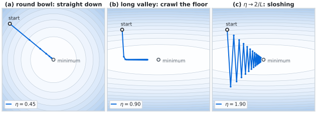
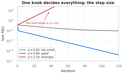
When the curvature is unknown, the classical remedy is a line search: try \(\eta=1\), halve it until the loss actually decreases, and repeat . Deep learning rarely does this, because every trial costs a full pass over the data; it schedules \(\eta\) by hand instead. Theory supplies the pace: for a convex \(L\)-smooth objective, gradient descent reaches \(f(\theta_t)-f^\star\le 2L\|\theta_0-\theta^\star\|^2/(t+1)\), that is, \(O(1/t)\) . Halving the distance to the optimum costs a doubling of iterations—a fair summary of why first-order methods need so many steps.
Nothing above said how to obtain \(g_t\). For a network with millions of weights there is no formula to differentiate by hand, and finite differences would cost one forward pass per parameter. Backpropagation computes all partial derivatives in a single backward sweep, using only the chain rule.
In a feed-forward network each layer alternates an affine map and an activation, \(a^{(\ell)}=W^{(\ell)}z^{(\ell-1)}+b^{(\ell)}\) and \(z^{(\ell)}=\sigma(a^{(\ell)})\). The forward pass stores every \(a\) and \(z\). The backward pass then propagates one number per neuron, \(\delta^{(\ell)}=\partial e/\partial a^{(\ell)}\), from the loss towards the input, \[\delta^{(L)} = \frac{\partial e}{\partial z^{(L)}}\odot\sigma'(a^{(L)}), \qquad \delta^{(\ell)} = \sigma'(a^{(\ell)})\odot \left(W^{(\ell+1)\top}\delta^{(\ell+1)}\right), \qquad \frac{\partial e}{\partial W^{(\ell)}} = \delta^{(\ell)}\,z^{(\ell-1)\top}, \label{eq:opt-tut-backprop}\] where \(\odot\) is the element-wise product. The gradient of a weight is therefore the product of a backward number and a forward number—the two quantities drawn in Figure 78. The recursion is linear in the layer index, so the whole sweep costs about the same as one extra forward pass, roughly twice the forward cost per step, and it must keep the activations of every layer in memory until they are used .
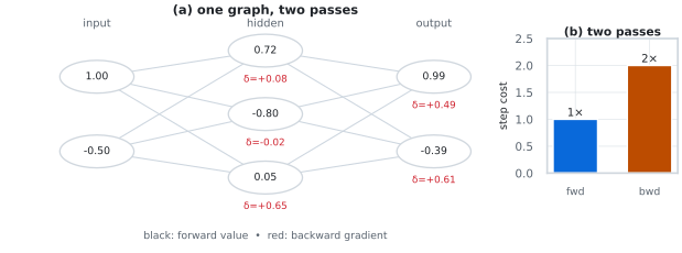
Input \(x\), target \(y\), weights \(\{W^{(\ell)},b^{(\ell)}\}_{\ell=1}^{L}\) Gradients \(\{\partial e/\partial W^{(\ell)}\}_{\ell=1}^{L}\) Forward: \(z^{(0)}\gets x\); for \(\ell=1,\dots,L\) do \(a^{(\ell)}\gets W^{(\ell)}z^{(\ell-1)}+b^{(\ell)}\), \(z^{(\ell)}\gets\sigma(a^{(\ell)})\) Loss: \(e \gets \ell(z^{(L)}, y)\) \(\delta^{(L)} \gets \partial e/\partial z^{(L)} \odot \sigma'(a^{(L)})\) \(\partial e/\partial W^{(\ell)} \gets \delta^{(\ell)} z^{(\ell-1)\top}\) \(\partial e/\partial b^{(\ell)} \gets \delta^{(\ell)}\) \(\delta^{(\ell-1)} \gets \sigma'(a^{(\ell-1)})\odot\left(W^{(\ell)\top}\delta^{(\ell)}\right)\) all weight gradients
The important consequence for this appendix is that backpropagation is not an optimizer. It is a gradient factory, and it always returns the exact gradient of whatever batch it was given. Every difference between the families that follow lives after the factory, in how \(u_t\) in [eq:opt-tut-generic] is formed.
With \(n\) examples the loss is an average, \(f(\theta)=\frac1n\sum_i f_i(\theta)\), so the exact gradient is an average of \(n\) per-example gradients and one step costs \(n\) backward passes. For a dataset of a billion tokens that is unaffordable, and it is also wasteful: neighbouring examples usually say almost the same thing about the parameters.
Stochastic gradient descent, in the line of the Robbins–Monro stochastic approximation , replaces the average by one term, \(\hat g_t=\nabla f_{i_t}(\theta_t)\) with \(i_t\) drawn uniformly, giving \[\theta_{t+1} = \theta_t - \eta_t\,\nabla f_{i_t}(\theta_t). \label{eq:opt-tut-sgd}\] The estimate is unbiased, \(\mathbb{E}[\hat g_t]=g_t\), so on average it points the right way; its error falls as \(\sigma/\sqrt{b}\) when a batch of \(b\) examples is used instead of one . Modern libraries call this mini-batch method “SGD” and almost never use \(b=1\): one pass over the data (an epoch) then contains \(\lfloor n/b\rfloor\) updates rather than one . Figure 79 shows both faces of the trade: with the same number of steps and the same step size, small batches wander, and the noise they inject is precisely the quantity that shrinks as \(1/\sqrt{b}\).
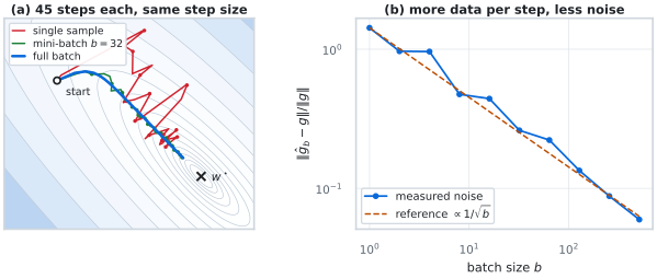
Noise is not only a cost. Because each step is a random approximation, the iterate can leave a shallow basin or slide across a saddle that a full-batch method would treat as a stopping point . The price appears in the rate. For a convex \(L\)-smooth objective, SGD with \(\eta_t\propto1/\sqrt t\) satisfies \(f(\theta_t)-f^\star=O(\log t/\sqrt t)\), and with a constant step it converges to a neighbourhood of size \(O(\eta)\) and then stalls . Full-batch gradient descent is therefore more accurate per iteration and much slower per iteration; SGD is the opposite. Figure 80 puts the two statements on the same axes, once per iteration and once per unit of wall-clock, which is the comparison that actually matters when a step costs \(n/b\) times less.
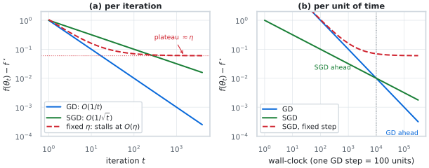
Everything after this point is a refinement of two observations about equation [eq:opt-tut-gd], and it is worth separating them before meeting the families.
A ball rolling down the same valley keeps its velocity: it accumulates speed along a consistent slope and cancels the oscillation when the slope keeps changing sign. Momentum implements exactly that, replacing the gradient by a decaying sum of gradients, \[v_t = \beta\,v_{t-1} - \eta\,g_t, \qquad \theta_{t+1} = \theta_t + v_t, \label{eq:opt-tut-momentum}\] with \(\beta\in[0,1)\) the decay. The effective step is \(\eta/(1-\beta)\) along a steady direction, which is how a small \(\eta\) can still move quickly. Nesterov momentum makes the same move but reads the gradient at the position the velocity is heading towards, so the correction arrives before the overshoot does . Figure 81 shows the composition of the two terms and its effect on the valley.
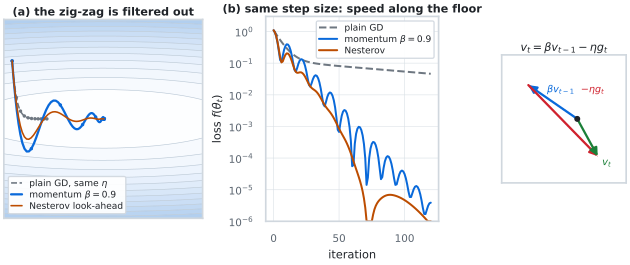
The second observation is that the valley of Figure 76(b) has no single good \(\eta\): what is stable along the steep axis is negligible along the flat one. Adaptive methods keep a running average of squared gradients and divide by its square root, so a coordinate that has been receiving large gradients gets a smaller step and a quiet coordinate gets a larger one, \[s_t = \gamma\,s_{t-1} + (1-\gamma)\,g_t^2, \qquad \theta_{t+1} = \theta_t - \eta\,\frac{g_t}{\sqrt{s_t}+\epsilon}. \label{eq:opt-tut-rms}\] The scheme grew out of rprop, which used only the sign of the gradient, and its mini-batch version, rmsprop ; AdaGrad is the cumulative rather than decaying version . Figure 82 shows the effect: the two axes of the valley receive comparable displacements, at the cost of a per-coordinate state and a step that no longer shrinks on its own—the residual jitter of size \(\approx\eta\) around the minimum is what later motivates decaying or schedule-free step sizes.
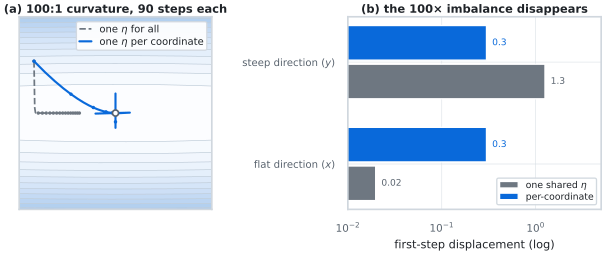
The two knobs compose, and their composition is the reason AdamW is the default in practice: a first moment for direction, a second moment for scale, a bias correction for the empty first steps, and a decoupled weight decay for regularisation . Nothing in equations [eq:opt-tut-momentum] and [eq:opt-tut-rms] is specific to transformers; what differs across the families is which statistics are kept, how they are combined, and how many bytes per parameter that costs. A compact survey of the resulting zoo is given by .
The appendix that follows contains thirty-eight methods, which is too many to hold in mind at once. They are easier to remember as eight families, each answering one of the questions in Figure 75 and each distinguished by what it remembers and what it pays.
First-order baselines (SGD with momentum, AdamW, RAdam) keep one or two statistics per parameter and assume the landscape is smooth enough for a locally linear model. They are the reference against which everything else is measured.
Momentum and variance reduction (Adan, ADOPT, AdEMAMix, MARS, Cautious AdamW) keep more than two buffers, or a gradient difference, to reduce the variance of the update itself. They buy stability and speed at the cost of memory and of a second gradient evaluation or a longer history.
Memory-efficient and low-rank (Adafactor, GaLore, APOLLO, Lion, AdamPM) accept a worse estimate of the second moment—a factored one, a projected one, or none—precisely to shrink the state. Lion goes as far as keeping only the sign of the update.
Schedule-free and parameter-free (Schedule-Free AdamW, Prodigy, LAMB for large batches) move the burden of choosing \(\eta_t\) from the practitioner to the algorithm, usually by averaging iterates or by estimating the step from the loss itself.
Curvature and second-order (Sophia, Shampoo, SOAP) estimate how the gradient changes, not just its size, and precondition the step with that estimate. They converge in fewer iterations and cost more per iteration.
Geometric and orthogonality (Muon, Turbo-Muon, AF-Muon, ROOT, NorMuon, Dion3) treat a weight matrix as a matrix: they orthogonalise or otherwise whiten the update so that all singular directions move at the same rate, which is a cheap surrogate for curvature on matrix-shaped parameters.
Adaptivity-tunable (Anon) keeps the standard state but adapts its own coefficients, so the amount of adaptivity is a hyperparameter rather than a fixed design choice.
Evolutionary and population (EvE, EA4LLM) do not follow a gradient at all: they sample perturbations or maintain a population of models, which is attractive when gradients are noisy, unavailable, or when many hyperparameters must be tuned at once, and expensive when the model is large.
Table [tab:opt-tut-families] states the same comparison in the two currencies that decide a real training run: what is stored per parameter and what each step costs. Figure 83 turns it into a fingerprint: reading down a row tells you which ingredients a family uses, reading across a column tells you which families share one.
@L3.2cmL4.6cmL2.6cmL4.6cm@
Family & Question answered & State per parameter & Main
risk
First-order baseline & What is the slope? & 0–2 & needs a
hand-tuned schedule
Momentum, variance reduction & Which way is it going? & 2–3
& more memory and bookkeeping
Memory-efficient, low-rank & Can the state be smaller? & \(\le1\) & biased second moment
Schedule-free, parameter-free & Can \(\eta_t\) be chosen for me? & 1 &
theory assumes convexity
Curvature, second-order & How does the slope change? & \(2+2k\) & expensive factorisations
Geometric, orthogonality & Is the update well shaped? & 1 &
matrices only
Adaptivity-tunable & How adaptive is it? & 2 & extra
hyperparameters
Evolutionary, population & Can we search without gradients? &
\(P\times\) & prohibitive at
scale
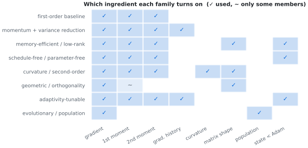
Algorithm [alg:opt-tut-generic] makes the comparison operational: the families differ only in which slots they fill. Reading it side by side with Table [tab:opt-tut-knobs] is enough to place any method from the rest of the appendix without memorising its algebra.
Parameters \(\theta_0\), learning rate \(\eta\), slots \(\mathcal{S}\) (state), \(\mathcal{D}\) (direction), \(\mathcal{P}\) (preconditioner), \(\mathcal{T}\) (step rule) Updated parameters \(\theta_T\) Initialize the state required by \(\mathcal{S}\) Sample a batch \(\mathcal{B}_t\) and compute \(g_t\gets\nabla f_{\mathcal{B}_t}(\theta_{t-1})\) Update the state: \(\mathcal{S}\gets\textsc{Update}(\mathcal{S}, g_t, \theta_{t-1})\) Form the direction \(u_t\gets\mathcal{D}(g_t,\mathcal{S})\) Apply the preconditioner \(u_t\gets\mathcal{P}(u_t,\mathcal{S})\) Choose the step \(\eta_t\gets\mathcal{T}(\eta, t, \mathcal{S})\) \(\theta_t\gets\theta_{t-1}-\eta_t\,u_t\) \(\theta_T\)
@L2.4cmL4.4cmL3.4cmL3.6cm@
Slot & What it decides & Knob turned & Seen in
\(\mathcal{B}_t\) & how many
examples per step & variance & SGD, mini-batch, full batch
\(\mathcal{S}\) & what is
remembered & state and memory & momentum, Adam, Sophia,
Shampoo
\(\mathcal{D}\) & which direction
is followed & smoothing & momentum, Nesterov, sign methods
\(\mathcal{P}\) & how coordinates
are rescaled & conditioning & AdaGrad, RMSProp, Adam, Muon
\(\mathcal{T}\) & how long the step
is & schedule & cosine, warmup, schedule-free, Prodigy
decay & how parameters are regularised & generalisation &
L2, decoupled weight decay
The practical value of the five ideas is diagnostic. A single loss curve already says which of them is wrong, and the answer is usually visible within a few hundred steps (Figure 84).
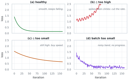
Five rules of thumb close the tutorial, all of them consequences of the figures above rather than of any particular method.
Start from a first-order baseline with both moments (AdamW). It is the cheapest configuration that survives heterogeneous curvature.
If the optimizer state does not fit in memory, change family before changing hyper parameters: the memory-efficient and low-rank families exist for exactly that constraint.
If tuning the schedule consumes the experiment budget, the schedule-free and parameter-free families remove the knob instead of tuning it.
If most parameters live in matrices (attention and feed-forward projections), geometric methods exploit a structure that element-wise methods ignore; if the model is small and the search is over many configurations, population methods become affordable.
Change one slot at a time. Because the families are orthogonal compositions, a run that changes two of them cannot attribute its result.
The rest of this appendix is the reference behind these statements: one entry per method, each stating its update rule, its pseudocode, its memory profile, and the trade it makes.

The plainest first-order method: update the weights with the gradient of the current mini-batch instead of the full batch . On redundant datasets the mini-batch gradient is nearly as informative as the full one, and computing it with matrix–matrix products makes it markedly cheaper than online updates, especially on GPUs. At iteration \(t\) with mini-batch \(B\): \[\begin{aligned} g_t &= \frac{1}{|B|} \sum_{i \in B} \nabla_\theta E_i(\theta_t) \\ \theta_{t+1} &= \theta_t - \eta\, g_t \end{aligned}\] where \(\eta\) is the only hyperparameter of the method. The deck’s own tuning recipe is heuristic: reduce the rate when the error oscillates or diverges, increase it when the error falls consistently but slowly, and turn it down towards the end of training . Momentum is a separate extension (next paragraph); this entry is deliberately the zero-state baseline of the catalog.
Initial parameters \(\theta_0\), learning rate \(\eta\), weight decay \(\lambda\) Updated parameters \(\theta_T\) Sample a mini-batch \(B_t\); compute \(g_t \gets \frac{1}{|B_t|}\sum_{i \in B_t}\nabla f_i(\theta_t)\) \(g_t \gets g_t + \lambda \theta_t\) Update parameters: \(\theta_{t+1} \gets \theta_t - \eta\, g_t\) \(\theta_T\)
A single global rate cannot suit heterogeneous curvature: the method zig-zags across narrow ravines and stalls along flat directions.
Strong dependence on hand-tuned learning-rate schedules; no per-parameter adaptivity.
Zero optimizer state: the memory floor of the catalog and the cheapest step.
Fully deterministic given the batch order; the reference point against which every other entry is measured.

The classical update accumulates a momentum buffer and then applies a fixed learning rate. At each iteration \(t\), the algorithm maintains an exponential moving average \(m_t\) of past gradients: \[\begin{aligned} m_t &= \beta m_{t-1} + g_t \\ \theta_{t+1} &= \theta_t - \eta m_t \end{aligned}\] where \(g_t = \nabla f(\theta_t)\), \(\beta \in [0.8, 0.99]\) controls the momentum decay, and \(\eta\) is the fixed learning rate. The momentum term acts as velocity: it accelerates movement in consistent directions while dampening oscillations in variable directions.
Initial parameters \(\theta_0\), learning rate \(\eta\), momentum coefficient \(\beta\), weight decay \(\lambda\) Updated parameters \(\theta_T\) Initialize: momentum buffer \(m \gets 0\) Compute gradient: \(g_t \gets \nabla f(\theta_t)\) \(g_t \gets g_t + \lambda \theta_t\) Update momentum: \(m \gets \beta \cdot m + g_t\) Update parameters: \(\theta_{t+1} \gets \theta_t - \eta \cdot m\) \(\theta_T\)
Poor robustness to heterogeneous curvature: a single global rate cannot suit every parameter group.
Strong dependence on carefully engineered learning-rate schedules.
Low memory overhead: a single momentum buffer per parameter.
Strong generalization when tuned carefully, and a simple update to implement.

RMSProp is the mini-batch-safe version of rprop: instead of dividing
by the size of the current gradient, force the divisor to be nearly
identical for adjacent mini-batches by keeping a moving average of the
squared gradient for each weight : \[\begin{aligned}
v_t &= 0.9\, v_{t-1} + 0.1\, g_t^2 \\
\theta_{t+1} &= \theta_t - \eta\, \frac{g_t}{\sqrt{v_t} + \epsilon}
\end{aligned}\] where \(g_t = \partial
E/\partial w(t)\), the \(0.9/0.1\) split is the exponential decay of
the slides (exposed as the alpha hyperparameter), and \(\epsilon\) is a numerical guard added by
the implementation (the slides define none). No bias correction and no
first moment appear in the original method ; combining it with momentum is
explicitly left open by the deck (“momentum does not help as much as it
normally does”). The running average is the only state buffer and the
direct predecessor of the adaptive family: AdaGrad’s diagonal idea made
mini-batch-safe, later extended into Adam.
Initial parameters \(\theta_0\), learning rate \(\eta\), decay \(\alpha = 0.9\), epsilon \(\epsilon\), weight decay \(\lambda\) Updated parameters \(\theta_T\) Initialize: running average \(v \gets 0\) Compute gradient: \(g_t \gets \nabla f(\theta_t)\) \(g_t \gets g_t + \lambda \theta_t\) Update running average: \(v \gets \alpha v + (1-\alpha) g_t^2\) Update parameters: \(\theta_{t+1} \gets \theta_t - \eta\, g_t / (\sqrt{v} + \epsilon)\) \(\theta_T\)
No bias correction: the divisor is inflated early in training, when \(v_t\) is still a poor estimate.
Still tuning-sensitive (rate, decay, epsilon) and largely superseded by Adam for transformers.
One buffer per parameter and an \(\mathcal{O}(n)\) step — the cheapest adaptive method in the catalog.
Per-coordinate scaling keeps the step robust to heterogeneous gradient magnitudes across layers.

Adam tracks exponential moving averages of both first moment (mean) and second moment (uncentered variance) to achieve element-wise adaptive learning rates. The update rule is: \[\begin{aligned} m_t &= \beta_1 m_{t-1} + (1-\beta_1) g_t \\ v_t &= \beta_2 v_{t-1} + (1-\beta_2) g_t^2 \\ \hat{m}_t &= \frac{m_t}{1-\beta_1^t}, \quad \hat{v}_t = \frac{v_t}{1-\beta_2^t} \quad \text{(bias correction)} \\ \theta_{t+1} &= \theta_t - \eta \left(\frac{\hat{m}_t}{\sqrt{\hat{v}_t}+\epsilon}\right) \end{aligned}\] AdamW introduces a crucial modification: weight decay is applied directly to parameters (decoupled from gradients): \(\theta_t \gets \theta_t(1-\eta\lambda)\) rather than adding \(\lambda\theta_t\) to the gradient. This decoupling prevents the adaptive scaling from interfering with regularization strength.
Initial parameters \(\theta_0\), learning rate \(\eta\), exponential decay rates \(\beta_1, \beta_2 \in [0,1)\) Momentum constant \(\epsilon\), weight decay \(\lambda\) Updated parameters \(\theta_T\) Initialize: first moment \(m \gets 0\), second moment \(v \gets 0\), step counter \(t \gets 0\) Compute gradient: \(g_t \gets \nabla f(\theta_{t-1})\) Weight decay (decoupled): \(\theta_{t-1} \gets \theta_{t-1}(1 - \eta\lambda)\) Update moments: \(m \gets \beta_1 m + (1-\beta_1) g_t\) \(v \gets \beta_2 v + (1-\beta_2) g_t^2\) Bias correction: \(\hat{m} \gets m / (1 - \beta_1^t)\), \(\hat{v} \gets v / (1 - \beta_2^t)\) Update parameters: \(\theta_t \gets \theta_{t-1} - \eta (\hat{m} / (\sqrt{\hat{v}} + \epsilon))\) \(\theta_T\)
Stores first and second moment tensors for every parameter, doubling optimizer-state memory relative to SGD.
Element-wise adaptive scaling can interfere with regularization unless weight decay is decoupled.
Practical baseline for transformer fine-tuning: fast convergence and forgiving to hyperparameter variation.
Decoupled weight decay keeps the regularization strength independent of the adaptive scaling.

RAdam addresses Adam’s instability in early training by dynamically rectifying the adaptive learning rate. The key observation is that the second moment \(v_t\) has very high variance in the first few steps, causing unreliable adaptive scaling. RAdam computes the effective simple moving average (SMA) window length: \[\rho_t = \rho_{\infty} - \frac{2t\beta_2^t}{1-\beta_2^t}, \quad \text{where} \quad \rho_{\infty} = \frac{2}{1-\beta_2}-1\] When \(\rho_t > 4\) (sufficient samples for variance estimation), RAdam applies adaptive scaling with a rectification term: \[r_t = \sqrt{\frac{(\rho_t-4)(\rho_t-2)\rho_{\infty}}{(\rho_{\infty}-4)(\rho_{\infty}-2)\rho_t}}, \quad \theta_{t+1} = \theta_t - \eta r_t \frac{\hat{m}_t}{\sqrt{\hat{v}_t}+\epsilon}\] When \(\rho_t \leq 4\), RAdam falls back to SGD with momentum: \(\theta_{t+1} = \theta_t - \eta\hat{m}_t\).
Initial parameters \(\theta_0\), learning rate \(\eta\), \(\beta_1, \beta_2\), weight decay \(\lambda\) Updated parameters \(\theta_T\) Initialize: \(m \gets 0\), \(v \gets 0\), \(t \gets 0\) Compute: \(\rho_\infty \gets 2/(1-\beta_2) - 1\) \(g_t \gets \nabla f(\theta_{t-1})\) \(\theta_{t-1} \gets \theta_{t-1}(1 - \eta\lambda)\) \(m \gets \beta_1 m + (1-\beta_1) g_t\) \(v \gets \beta_2 v + (1-\beta_2) g_t^2\) \(\hat{m} \gets m/(1-\beta_1^t)\), \(\hat{v} \gets v/(1-\beta_2^t)\) \(\rho_t \gets \rho_\infty - 2t \beta_2^t / (1 - \beta_2^t)\) \(r_t \gets \sqrt{((\rho_t-4)(\rho_t-2)\rho_\infty) / ((\rho_\infty-4)(\rho_\infty-2)\rho_t)}\) \(\theta_t \gets \theta_{t-1} - \eta r_t \hat{m} / (\sqrt{\hat{v}} + \epsilon)\) \(\theta_t \gets \theta_{t-1} - \eta \hat{m}\) \(\theta_T\)
Adds rectification bookkeeping on top of Adam’s moment state.
The benefit shrinks when a well-tuned warmup schedule is already in use.
Eliminates the need for manual learning-rate warmup by rectifying the adaptive rate.
Falls back gracefully to momentum SGD while variance estimates are unreliable, improving robustness.
LaProp targets an unnecessary coupling in Adam rather than a new preconditioner . Writing the adaptive family as \(\theta_{t+1} = \theta_t - \lambda_t G_t \nabla\ell(\theta_t) + \mu_t K_t(\theta_t - \theta_{t-1})\), Adam’s parameter-space momentum is multiplied by \(K_t = H_t^{-1}H_{t-1}\), i.e. the previous motion is rescaled by the current preconditioner. A single pathologically large gradient—noise, an out-of-distribution batch, or an explosion—can therefore erase the accumulated momentum. LaProp simply sets \(K_t = I\) and instead accumulates the momentum of the preconditioned gradient: \[\begin{aligned} n_t &= \nu n_{t-1} + (1-\nu) g_t^2 \\ m_t &= \mu m_{t-1} + (1-\mu)\,\frac{g_t}{\sqrt{n_t/(1-\nu^t)} + \epsilon} \\ \theta_{t+1} &= \theta_t - \lambda\,\frac{m_t}{1-\mu^t} \end{aligned}\] with \(g_t = \nabla\ell(\theta_t)\) and \(0 \le \mu, \nu < 1\). The second moment \(n_t\) is Adam’s uncentered variance; the first moment \(m_t\) averages the already-normalized direction, so the parameter-space momentum stays additive like SGD. The influence of any single gradient on the accumulated momentum is bounded by \((1-\mu)/\sqrt{1-\nu}\). LaProp has exactly the state (two buffers), per-step cost and hyperparameter count of Adam, and Adam’s settings carry over unchanged; \(\nu \to 0\) recovers signed-gradient methods and \(\mu = 0\) recovers RMSProp with bias correction (the paper describes it as RMSProp with momentum plus both correction factors).
Initial parameters \(\theta_1\), learning rate \(\{\lambda_t\}_{t=1}^T\), decay parameters \(0 \le \mu, \nu < 1\) Epsilon \(\epsilon \ll 1\), weight decay \(\lambda_{\mathrm{wd}}\) Updated parameters \(\theta_T\) Initialize: first moment \(m_0 \gets 0\), second moment \(n_0 \gets 0\) \(g_t \gets \nabla_\theta \ell(\theta_t)\) \(g_t \gets g_t + \lambda_{\mathrm{wd}} \theta_t\) \(n_t \gets \nu n_{t-1} + (1-\nu) g_t^2\) \(m_t \gets \mu m_{t-1} + (1-\mu) g_t / (\sqrt{n_t/(1-\nu^t)} + \epsilon)\) \(\theta_{t+1} \gets \theta_t - \lambda_t\, m_t / (1-\mu^t)\) \(\theta_T\)
Does not dominate Adam on every task; its gains are concentrated in noisy or unstable optimization regimes.
Couples the momentum decay to the preconditioned scale, so the effective step size at initialization differs from Adam until the bias correction settles.
Adam-identical memory (\(m\), \(v\)), per-step cost and hyperparameter count; existing Adam settings transfer directly.
Keeps parameter-space momentum additive, avoiding the \(H_t^{-1}H_{t-1}\) reweighting that lets one bad gradient wipe the accumulated direction.
Interpolates continuously between adaptive and signed-gradient updates through \(\nu\).

Adan reformulates Nesterov acceleration without the extra gradient computation required by classical Nesterov SGD. The algorithm maintains three momentum buffers: \[\begin{aligned} m_t &= (1-\beta_1)m_{t-1} + \beta_1 g_t \quad\text{(first moment)} \\ v_t &= (1-\beta_2)v_{t-1} + \beta_2(g_t - g_{t-1}) \quad\text{(velocity/gradient difference)} \\ n_t &= (1-\beta_3)n_{t-1} + \beta_3[g_t + (1-\beta_1)(g_t-g_{t-1})]^2 \quad\text{(Nesterov second moment)} \end{aligned}\] The Nesterov Momentum Estimation (NME) term \(\bar{g}_t = g_t + (1-\beta_1)(g_t-g_{t-1})\) estimates the gradient at a future position without evaluating it. The update combines momentum with velocity: \[\bar{m}_t = m_t + (1-\beta_1)v_t, \quad \theta_{t+1} = \theta_t - \eta\frac{\bar{m}_t}{\sqrt{n_t}+\epsilon}\]
Initial parameters \(\theta_0\), learning rate \(\eta\), \(\beta_1, \beta_2, \beta_3 \in (0,1)\) Updated parameters \(\theta_T\) Initialize: \(m \gets 0\), \(v \gets 0\), \(n \gets 0\), \(g_{-1} \gets 0\) (previous gradient) \(g_t \gets \nabla f(\theta_{t-1})\) \(m \gets (1-\beta_1) m + \beta_1 g_t\) \(\Delta g_t \gets g_t - g_{t-1}\) \(v \gets (1-\beta_2) v + \beta_2 \Delta g_t\) Nesterov estimation: \(\bar{g}_t \gets g_t + (1-\beta_1) \Delta g_t\) \(n \gets (1-\beta_3) n + \beta_3 \bar{g}_t^2\) Combined momentum: \(\bar{m} \gets m + (1-\beta_1) v\) \(\theta_t \gets \theta_{t-1} - \eta (\bar{m} / (\sqrt{n} + \epsilon))\) \(g_{t-1} \gets g_t\) \(\theta_T\)
Three momentum-like buffers increase memory overhead relative to Adam.
Additional gradient-difference bookkeeping per step.
Nesterov-style acceleration without an extra gradient evaluation.
Fast convergence across diverse architectures (CNNs, GANs, transformers).

ADOPT fixes a fundamental theoretical issue in Adam: the gradient appears in both the first moment and second moment estimates, creating circularity. ADOPT decouples by using the previous step’s second moment for the denominator: \[\begin{aligned} v_t &= \beta_2 v_{t-1} + (1-\beta_2)g_t^2 \\ m_t &= \beta_1 m_{t-1} + (1-\beta_1)\frac{g_t}{\sqrt{v_{t-1}}+\epsilon} \quad\text{(uses $v_{t-1}$, not $v_t$)} \\ \theta_{t+1} &= \theta_t - \eta m_t \end{aligned}\]
Initial parameters \(\theta_0\), learning rate \(\eta\), \(\beta_1, \beta_2\), tolerance \(\epsilon\) Updated parameters \(\theta_T\) Initialize: \(m \gets 0\), \(v \gets 0\) \(g_t \gets \nabla f(\theta_{t-1})\) \(\theta_{t-1} \gets \theta_{t-1}(1 - \eta\lambda)\) Use previous second moment: \(\text{denom} \gets \sqrt{\max(v, \epsilon)} + \epsilon\) Update first moment using previous variance: \(m \gets \beta_1 m + (1-\beta_1)(g_t / \text{denom})\) Update second moment with current gradient: \(v \gets \beta_2 v + (1-\beta_2) g_t^2\) \(\theta_t \gets \theta_{t-1} - \eta m\) \(\theta_T\)
Requires keeping the previous second moment as an explicit denominator.
Empirical gains are architecture- and tuning-dependent.
Removes Adam’s gradient circularity and attains the optimal convergence rate \(O(1/\sqrt{T})\) with any \(\beta_2 \in (0,1)\), without bounded-noise assumptions.
Drop-in Adam replacement with comparable or superior empirical performance across vision, NLP, RL, and generative modeling.

AdEMAMix replaces Adam’s single EMA of gradients with a mixture of two EMAs: one fast-decaying and one slow-decaying. This addresses the observation that gradients remain informative over tens of thousands of steps, not just hundreds: \[\begin{aligned} m_{1,t} &= \beta_1 m_{1,t-1} + (1-\beta_1)g_t \quad\text{(fast EMA, $\beta_1 \approx 0.9$)} \\ m_{2,t} &= \beta_3 m_{2,t-1} + (1-\beta_3)g_t \quad\text{(slow EMA, $\beta_3 \approx 0.9999$)} \\ v_t &= \beta_2 v_{t-1} + (1-\beta_2)g_t^2 \\ m_t &= m_{1,t} + \alpha_t m_{2,t} \quad\text{(mixture with scheduled weight $\alpha_t$)} \\ \theta_{t+1} &= \theta_t - \eta\frac{m_t}{\sqrt{v_t}+\epsilon} \end{aligned}\] The mixture weight \(\alpha_t\) typically increases during training, allowing the fast EMA to provide immediate adaptation while the slow EMA accumulates long-range gradient correlations.
Initial parameters \(\theta_0\), learning rate \(\eta\), \(\beta_1\) (fast), \(\beta_3\) (slow), \(\beta_2\) (second moment) Mixture weight \(\alpha_t\) (typically increasing), tolerance \(\epsilon\) Updated parameters \(\theta_T\) Initialize: \(m_1 \gets 0\) (fast EMA), \(m_2 \gets 0\) (slow EMA), \(v \gets 0\) \(g_t \gets \nabla f(\theta_{t-1})\) \(\theta_{t-1} \gets \theta_{t-1}(1 - \eta\lambda)\) \(m_1 \gets \beta_1 m_1 + (1-\beta_1) g_t\) \(m_2 \gets \beta_3 m_2 + (1-\beta_3) g_t\) \(v \gets \beta_2 v + (1-\beta_2) g_t^2\) \(m_t \gets m_1 + \alpha_t m_2\) \(\theta_t \gets \theta_{t-1} - \eta (m_t / (\sqrt{v} + \epsilon))\) \(\theta_T\)
Two gradient EMAs plus the second moment roughly triple Adam’s optimizer state.
The mixture schedule \(\alpha_t\) adds a hyperparameter to tune.
Exploits gradient information that remains informative over tens of thousands of steps.
A 1.3B model on 101B tokens matches AdamW on 197B tokens (95% data-efficiency gain), suggesting reduced forgetting.

MARS combines preconditioned gradient methods (e.g., AdamW) with variance reduction via scaled stochastic recursive momentum. The core innovation is a variance-reduced gradient estimate: \[\begin{aligned} c_t &= g_t + \gamma(c_{t-1} - g_{t-1}) \quad\text{(SVRG-style recursive estimate)} \\ m_t &= \beta_1 m_{t-1} + (1-\beta_1)c_t \\ v_t &= \beta_2 v_{t-1} + (1-\beta_2)c_t^2 \\ \theta_{t+1} &= \theta_t - \eta\frac{m_t}{\sqrt{v_t}+\epsilon} \end{aligned}\] where \(\gamma \in [0.01, 0.1]\) controls how much historical gradient information is retained. The variance-reduced gradient \(c_t\) acts as an implicit noise filter, amplifying consistent signal directions and dampening contradictory noise.
Initial parameters \(\theta_0\), learning rate \(\eta\), \(\beta_1, \beta_2\), weight decay \(\lambda\) Variance reduction coefficient \(\gamma \in [0.01, 0.1]\) Updated parameters \(\theta_T\) Initialize: \(m \gets 0\), \(v \gets 0\), \(c \gets 0\) (variance-reduced gradient), \(g_{-1} \gets 0\) \(g_t \gets \nabla f(\theta_{t-1})\) Variance reduction: \(c \gets g_t + \gamma(c - g_{t-1})\) \(m \gets \beta_1 m + (1-\beta_1) c\) \(v \gets \beta_2 v + (1-\beta_2) c^2\) \(\theta_{t-1} \gets \theta_{t-1}(1 - \eta\lambda)\) \(\theta_t \gets \theta_{t-1} - \eta (m / (\sqrt{v} + \epsilon))\) \(g_{t-1} \gets g_t\) \(\theta_T\)
Stores the variance-reduced gradient and the previous gradient in addition to Adam’s moments.
The variance-reduction coefficient \(\gamma \in [0.01, 0.1]\) must be tuned.
Acts as an implicit noise filter, amplifying consistent directions and dampening contradictory noise.
MARS-AdamW consistently outperforms bare AdamW by significant margins on GPT-2 pretraining.

The Cautious framework applies a one-line modification to any momentum-based optimizer: mask the update so that only dimensions where momentum and gradient directions agree are applied: \[\begin{aligned} \text{mask}_i &= \begin{cases} 1 & \text{if } m_t[i] \cdot g_t[i] > 0 \quad\text{(agreement)} \\ 0 & \text{otherwise} \end{cases} \\ u_t &= \left(\frac{m_t}{\sqrt{v_t}+\epsilon}\right) \odot \text{mask} \quad\text{(element-wise masking)} \\ \theta_{t+1} &= \theta_t - \eta u_t \end{aligned}\] The intuition: momentum \(m_t\) estimates the gradient direction from history; the current gradient \(g_t\) is instantaneous signal. When both agree, the optimizer is confident and should update aggressively. When they disagree, the optimizer is conflicted—the historical trend points toward a region that may have been good before, but current evidence contradicts it. By masking conflicted dimensions, Cautious becomes more conservative and avoids corrupted steps.
Initial parameters \(\theta_0\), learning rate \(\eta\), \(\beta_1, \beta_2\), weight decay \(\lambda\) Updated parameters \(\theta_T\) Initialize: \(m \gets 0\), \(v \gets 0\) \(g_t \gets \nabla f(\theta_{t-1})\) \(m \gets \beta_1 m + (1-\beta_1) g_t\) \(v \gets \beta_2 v + (1-\beta_2) g_t^2\) Consensus mask: \(\text{mask}_i \gets 1\) if \(m[i] \cdot g_t[i] > 0\), else \(0\) Base Adam update: \(u \gets m / (\sqrt{v} + \epsilon)\) Apply mask: \(u_{\text{masked}} \gets u \odot \text{mask}\) \(\theta_{t-1} \gets \theta_{t-1}(1 - \eta\lambda)\) \(\theta_t \gets \theta_{t-1} - \eta u_{\text{masked}}\) \(\theta_T\)
Masking can discard useful updates when momentum and gradient temporarily disagree.
Requires a base momentum optimizer plus the element-wise mask.
A one-line modification applicable to any momentum-based optimizer.
Up to 1.47\(\times\) speedup on Llama and MAE pretraining while preserving convergence guarantees.

LAMB extends Adam with layer-wise adaptive rate scaling (inspired by LARS), enabling stable training with extreme batch sizes (e.g., 64K on BERT): \[\begin{aligned} m_t^L &= \beta_1 m_{t-1}^L + (1-\beta_1)g_t^L \quad\text{(layer-wise first moment)} \\ v_t^L &= \beta_2 v_{t-1}^L + (1-\beta_2)(g_t^L)^2 \\ u_{\text{adam}}^L &= \frac{m_t^L}{\sqrt{v_t^L}+\epsilon} + \lambda\theta_{t-1}^L \quad\text{(base adaptive step with decay)} \\ \phi^L &= \frac{\|\theta_{t-1}^L\|_2}{\|u_{\text{adam}}^L\|_2} \quad\text{(trust ratio: layer normalization)} \\ \theta_t^L &= \theta_{t-1}^L - \eta \cdot \phi^L \cdot u_{\text{adam}}^L \end{aligned}\] The trust ratio \(\phi^L = \|\theta^L\|_2 / \|u_{\text{adam}}^L\|_2\) normalizes the effective update step relative to weight magnitude. In very large batches, stochastic gradient noise can exceed signal, destabilizing layer-wise learning rates. By scaling updates proportionally to weight norms, LAMB ensures relative changes rather than absolute ones, preventing small confident updates in large vectors from dominating.
Initial parameters \(\theta_0\), learning rate \(\eta\), \(\beta_1, \beta_2\), weight decay \(\lambda\) Updated parameters \(\theta_T\) Initialize: For each layer \(L\): \(m^L \gets 0\), \(v^L \gets 0\) \(g_t^L \gets \nabla f(\theta_t^L)\) \(m^L \gets \beta_1 m^L + (1-\beta_1) g_t^L\) \(v^L \gets \beta_2 v^L + (1-\beta_2) (g_t^L)^2\) Base Adam: \(u_{\text{adam}}^L \gets m^L / (\sqrt{v^L} + \epsilon)\) \(u_{\text{adam}}^L \gets u_{\text{adam}}^L + \lambda \theta_{t-1}^L\) Trust ratio: \(\phi^L \gets \|\theta_{t-1}^L\|_2 / \|u_{\text{adam}}^L\|_2\) if both nonzero, else \(1\) \(\theta_t^L \gets \theta_{t-1}^L - \eta \phi^L u_{\text{adam}}^L\) \(\theta_T\)
Layer-wise norm bookkeeping and trust-ratio computation add per-step overhead.
The trust ratio is unstable when layer or update norms are close to zero.
Enables stable training with extreme batch sizes (e.g., 64K on BERT).
Preserves small-batch generalization benefits while scaling the batch.

Schedule-free methods remove explicit scheduler design from the optimization recipe. The algorithm maintains two parameter streams: \(z_t\) (exploration) and \(x_t\) (smooth average): \[\begin{aligned} v_t &= \beta_2 v_{t-1} + (1-\beta_2)g_t^2 \quad\text{(variance)} \\ z_t &= z_{t-1}(1-\eta\lambda) - \eta\frac{g_t}{\sqrt{v_t}+\epsilon} \quad\text{(adaptive step with decay)} \\ c_t &= \frac{1}{t+1} \quad\text{(averaging coefficient, decreases over time)} \\ x_t &= (1-c_t)x_{t-1} + c_t z_t \quad\text{(iterate averaging)} \\ y_t &= (1-\beta)z_t + \beta x_t \quad\text{(interpolation for evaluation point)} \end{aligned}\] The averaging coefficient \(c_t = 1/(t+1)\) implements an implicit learning-rate schedule without explicitly specifying total steps \(T\). This framework unifies scheduling and iterate averaging: the algorithm explores via \(z_t\) while accumulating stable direction via \(x_t\). The evaluation point \(y_t\) (used for gradient computation) interpolates between exploration and stability.
Initial parameters \(\theta_0\), learning rate \(\eta\) (fixed), \(\beta_1, \beta_2\), weight decay \(\lambda\) Updated parameters \(\theta_T\) or averaging \(x_T\) Initialize: \(z \gets \theta_0\) (exploration), \(x \gets \theta_0\) (average), \(v \gets 0\), \(t \gets 0\) \(g_t \gets \nabla f(y_{t-1})\) (gradient at interpolation point) \(v \gets \beta_2 v + (1-\beta_2) g_t^2\) Weight decay on \(z\): \(z \gets z(1 - \eta\lambda)\) \(z \gets z - \eta g_t / (\sqrt{v} + \epsilon)\) \(c_t \gets 1 / (t+1)\) \(x \gets (1-c_t) x + c_t z\) \(y_t \gets (1-\beta_1) z + \beta_1 x\) \(x_T\) or \(y_T\)
Maintains two parameter streams (\(z\) and \(x\)) and requires explicit handling of the evaluation point.
Behavior departs from scheduled baselines, which complicates comparisons.
Removes the explicit learning-rate schedule and its total-step hyperparameter.
State-of-the-art convergence across convex optimization, large-scale deep learning, and reinforcement learning.

Adafactor reduces optimizer memory by factorizing second-moment statistics for matrix-shaped parameters, storing only row and column accumulators rather than dense variance states. For a gradient matrix \(G_t \in \mathbb{R}^{m \times n}\): \[\begin{aligned} R_t &= \beta_2 R_{t-1} + (1-\beta_2)(G_t^2) \mathbf{1}_n^T \quad\text{(row variance)} \\ C_t &= \beta_2 C_{t-1} + (1-\beta_2) \mathbf{1}_m^\top (G_t^2) \quad\text{(column variance)} \\ \hat{V}_t &= \frac{R_t C_t}{\mathbf{1}_n^\top R_t} \quad\text{(reconstructed variance via outer product)} \\ U_t &= \frac{G_t}{\sqrt{\hat{V}_t}+\epsilon} \quad\text{(normalized adaptive step)} \\ \hat{U}_t &= \frac{U_t}{\max(1, \text{RMS}(U_t))} \quad\text{(stability clipping)} \end{aligned}\]
Gradient matrix \(G_t \in \mathbb{R}^{m \times n}\), learning rate \(\eta\), \(\beta_2 \approx 0.999\) Updated parameters \(\theta_T\) Initialize: Row accumulators \(R \gets \epsilon \mathbf{1}^T_m\), Column \(C \gets \epsilon \mathbf{1}_n\) \(G_t \gets \nabla f(\theta_t)\) (matrix gradient) \(R \gets \beta_2 R + (1-\beta_2) (G_t^2) \mathbf{1}_n^T\) \(C \gets \beta_2 C + (1-\beta_2) \mathbf{1}_m^\top (G_t^2)\) Reconstructed variance: \(\hat{V} \gets (R \cdot C) / (\mathbf{1}_n^\top R)\) Normalized adaptive step: \(U_t \gets G_t / (\sqrt{\hat{V}} + \epsilon)\) Per-row RMS clipping: \(\hat{U}_t \gets U_t / \max(1, \text{RMS}(U_t))\) \(\theta_{t+1} \gets \theta_t - \eta \hat{U}_t\) \(\theta_T\)
Factorized variance is an approximation and can be unstable on some tasks.
Reduced optimization expressiveness relative to full Adam.
Memory drops from \(O(n_{\text{params}})\) to \(O(\sqrt{n_{\text{params}}})\) for matrix parameters.
Most attractive when VRAM is dominated by optimizer state rather than activations.

GaLore projects 2D gradients into a low-rank subspace before optimization, reducing optimizer-state memory while maintaining adaptive step scaling. For a 2D parameter matrix \(W \in \mathbb{R}^{m \times n}\): \[\begin{aligned} U, S, V &= \text{SVD}(G_t) \quad\text{(compute singular decomposition)} \\ P &\in \mathbb{R}^{n \times r} \quad\text{or} \quad P^\top \in \mathbb{R}^{r \times m} \quad\text{(select top-$r$ singular vectors)} \\ G_{\text{low}} &= P^\top G_t \quad\text{(project to low-rank space)} \\ \Delta_{\text{low}} &= \text{Adam}(G_{\text{low}}) \quad\text{(optimize in compressed space)} \\ \Delta &= P \Delta_{\text{low}} \quad\text{(reconstruct in original space)} \end{aligned}\] By projecting into a rank-\(r\) subspace (typically \(r \ll \min(m,n)\)), optimizer state is reduced from \(O(mn)\) to \(O(r(m+n))\) for 2D parameters. This complementary memory-saving approach is especially relevant when the model is too large for full-rank optimizer state.
2D parameter matrix \(W \in \mathbb{R}^{m \times n}\), learning rate \(\eta\), rank \(r \ll \min(m,n)\) Updated parameters \(\theta_T\) Initialize: Adam state in low-rank space (if rank-2 variant) \(G_t \gets \nabla f(W_t)\) \(U_t, S_t, V_t^\top \gets \text{SVD}(G_t)\) (full or thin) Select projection: \(P \gets U_t[:, :r]\) or \(P \gets V_t[:, :r]\) Project gradient: \(G_{\text{low}} \gets P^\top G_t\) (or \(G_t P^\top\) for right projection) Run Adam on low-rank: \(\Delta_{\text{low}} \gets \text{Adam}(G_{\text{low}})\) Reconstruct in original space: \(\Delta \gets P \Delta_{\text{low}}\) (or \(\Delta_{\text{low}} P^\top\)) \(W_t \gets W_t - \eta \Delta\) \(\theta_T\)
Periodic SVD adds compute and introduces a projection-refresh interval to tune.
Low-rank projection can discard gradient information.
Optimizer state reduced from \(O(mn)\) to \(O(r(m+n))\) for 2D parameters.
Works synergistically with other techniques and has shown strong results on billion-parameter models.

The APOLLO family begins from the observation that AdamW’s element-wise denominator can be coarsened into a structured learning-rate update. Rather than storing dense moments for every parameter entry, APOLLO projects a matrix gradient \(G_t \in \mathbb{R}^{m \times n}\) into a compact random subspace and tracks Adam-style moments there: \[\begin{aligned} R_t &= P_t G_t \quad\text{or}\quad R_t = G_t P_t^\top \\ M_t^R &= \beta_1 M_{t-1}^R + (1-\beta_1)R_t \\ V_t^R &= \beta_2 V_{t-1}^R + (1-\beta_2)R_t^2 \\ \widetilde{R}_t &= \frac{M_t^R}{\sqrt{V_t^R}+\epsilon} \end{aligned}\] The projected state is not expanded back into a dense low-rank update as in SVD-based methods. Instead, APOLLO estimates a structured scaling tensor \(S_t\) in the original space. In the standard APOLLO variant, that scaling is channel-wise: each row or channel receives its own norm ratio. In APOLLO-Mini, the scaling is reduced to a single tensor-wise scalar, corresponding to the rank-1 extreme described in the paper. The resulting parameter update is therefore Adam-like in adaptation but much closer to SGD in state cost: \[W_t \gets (1-\eta\lambda)W_{t-1} - \eta\,\alpha\,(G_t \odot S_t)\] where \(\alpha\) is the extra scale factor used to stabilize highly compressed variants.
Weight matrix \(W \in \mathbb{R}^{m \times n}\) with \(m \le n\), learning rate \(\eta\), scale factor \(\alpha\), decay rates \((\beta_1, \beta_2)\), weight decay \(\lambda\), rank \(r\), projection refresh interval \(T\) Updated parameters \(W_T\) Initialize projected moments: \(M^R \gets 0\), \(V^R \gets 0\), step \(t \gets 0\) Compute gradient: \(G_t \gets \nabla_W \phi(W_t)\) Sample Gaussian projector \(P_t \sim \mathcal{N}(0, 1/r)\) with a fresh seed Project gradient: \(R_t \gets P_t G_t\) Update projected AdamW moments: \(M_t^R, V_t^R \gets \text{AdamWState}(R_t; \beta_1, \beta_2)\) Normalize projected state: \(\widetilde{R}_t \gets M_t^R / (\sqrt{V_t^R}+\epsilon)\) \(S_t \gets \operatorname{diag}(s_1^R, \ldots, s_m^R)\), where \(s_i^R = \|\widetilde{R}_t[i,:]\|_2 / \|R_t[i,:]\|_2\) \(S_t \gets s_t^R\), where \(s_t^R = \|\widetilde{R}_t\|_2 / \|R_t\|_2\) Update weights: \(W_t \gets (1-\eta\lambda)W_{t-1} - \eta\,\alpha\,(G_t \odot S_t)\) \(t \gets t+1\)
Structured scaling is a coarser approximation of AdamW’s element-wise denominator.
Projectors must be refreshed periodically, and very small ranks make the scaling noisy.
Replaces repeated SVD with periodically refreshed Gaussian random projection, so the systems cost is ordinary matrix multiplication rather than spectral decomposition.
Unusually tolerant to extreme compression: even APOLLO-Mini, which keeps only rank-1 auxiliary state, remains competitive with or better than AdamW while approaching SGD-level memory.
APOLLO-Mini is the family member optimized for extreme memory efficiency. The paper motivates it by arguing that, in a rank-1 compact space, channel-wise scaling becomes too noisy, so the update is coarsened further to a single tensor-wise scale. The loss of granularity is partially offset by the explicit scaling factor \(\alpha\) (the paper discusses values such as \(128\) in this regime), giving a useful point on the optimization Pareto frontier: very small state, no SVD overhead, and still strong pre-training behavior.
A single tensor-wise scale loses channel granularity, and rank-1 state can be noisy.
Depends on the extra scale factor \(\alpha\) (e.g., \(128\)) to remain stable.
Smallest state in the APOLLO family, with no SVD overhead.
Strong pre-training behavior at near-SGD memory cost.
The APOLLO paper also stresses that the family combines naturally
with quantization for ultra-low-memory training. This
repository turns that systems observation into a concrete optimizer
variant, q_apollo. In the implementation, APOLLO’s low-rank
first and second moments are stored in quantized form together with
per-tensor scales and offsets, and are dequantized only when needed for
the next step. Q-APOLLO therefore preserves APOLLO’s projected-gradient
logic while reducing the precision of the remaining optimizer state.
Quantized moments introduce approximation error and dequantization overhead.
Requires managing per-tensor scales and offsets.
Reduces the remaining optimizer state to ultra-low precision.
Most aggressive memory-saving member of the local optimizer stack while preserving APOLLO’s projected-gradient logic.
AdamPM is a minimal, model-agnostic modification of Adam: it keeps the element-wise first moment untouched and compresses only the second moment by group-mean pooling of adjacent entries along each row (the default, rows being output features) or each column (the paper’s AdamPM-col). For a weight matrix \(W \in \mathbb{R}^{m \times n}\) and group size \(s\), every row is partitioned into \(q = \lceil n/s \rceil\) groups, the squared gradient is averaged within each group before the exponential moving average, and only the compressed statistic \(\bar{V}_t \in \mathbb{R}^{m \times q}\) is persisted: \[\begin{aligned} M_t &= \beta_1 M_{t-1} + (1-\beta_1)\, G_t && \text{(first moment, element-wise, Eq.~1)} \\ \bar{S}_t &= \frac{1}{s}\sum_{k=1}^{s} \mathrm{reshape}(G_t \odot G_t,\, m, q, s)[:,:,k] && \text{(within-group means, Eq.~2)} \\ \bar{V}_t &= \beta_2 \bar{V}_{t-1} + (1-\beta_2)\, \bar{S}_t && \text{(compressed second-moment EMA, Eq.~3)} \\ W_t &= W_{t-1} - \eta_t \, \frac{M_t/(1-\beta_1^t)} {\sqrt{\hat{\bar{V}}_t \otimes \mathbf{1}_{1\times s}} + \epsilon}, \qquad \hat{\bar{V}}_t = \frac{\bar{V}_t}{1-\beta_2^t} && \text{(update, Eq.~4)} \end{aligned}\] When \(n\) is not divisible by \(s\) the final group is padded with its own mean, so its statistic averages only the entries it actually contains; \(s{=}1\) recovers Adam exactly, and \(s \ge n\) collapses each row (or column) to one scalar, the paper’s AdamPM-inf limit. AdamPM pools the second moments of all weight matrices—embeddings, the LM head, attention and MLP weights—and treats one-dimensional parameters such as RMSNorm scales as single-row or single-column matrices, so no parameter group is left on a fallback path. The persistent state is \(mn(1+1/s)\) elements against Adam’s \(2mn\).
Initial parameters \(W_0 \in \mathbb{R}^{m\times n}\), steps \(T\), group size \(s\), learning rate \(\eta_t\), decay rates \(\beta_1, \beta_2\), stability constant \(\epsilon\) Updated parameters \(W_T\) \(t \gets 0\); \(q \gets \lceil n/s \rceil\) \(M_0 \gets \mathbf{0}_{m\times n}\); \(\bar{V}_0 \gets \mathbf{0}_{m\times q}\) \(t \gets t + 1\) \(G_t \gets \nabla_W \mathcal{L}(W_{t-1})\) \(M_t \gets \beta_1 M_{t-1} + (1-\beta_1) G_t\) \(\bar{S}_t \gets \operatorname{mean}_{k}\big(\mathrm{reshape}(G_t \odot G_t, m, q, s)[:,:,k]\big)\) \(\bar{V}_t \gets \beta_2 \bar{V}_{t-1} + (1-\beta_2) \bar{S}_t\) \(\hat{M}_t \gets M_t/(1-\beta_1^t)\); \(\hat{\bar{V}}_t \gets \bar{V}_t/(1-\beta_2^t)\) broadcast \(\hat{\bar{V}}_t\) over each group \(W_t \gets W_{t-1} - \eta_t \hat{M}_t / (\sqrt{\hat{\bar{V}}_t} + \epsilon)\) \(W_t\)
Empirically, AdamPM matches a carefully tuned Adam on LLaMA
pre-training from 60M to 1.3B parameters while cutting second-moment
memory by 87.5% (\(s{=}8\)) to 93.75%
(\(s{=}16\)), with the same pattern on
GLUE fine-tuning of RoBERTa-base and on TinyLLaVA-1B supervised
fine-tuning; group sizes between 2 and 8 are reported as robust, and
three or five—not only powers of two—work because the incomplete final
group is averaged over its own entries. Theorem 3.1 gives a stationarity
bound independent of the group size \(s\), and under a relative-noise condition
AdamPM attains the same \(\mathcal{O}(\log
T/\sqrt{T})\) rate as Adam. Algorithm 1 of the paper defines no
weight decay; this implementation applies the repository’s decoupled
wd_ decay before the adaptive update, and the shared
per-group betas/eps suffixes parameterize the
bias corrections and the denominator.
The diagonal preconditioner becomes coarser as \(s\) grows; the paper’s AdamPM-inf limit shows a measurable perplexity loss at 350M and 1.3B.
The saving covers optimizer state only: the first moment stays full-size, so optimizer memory is \(1+1/s\) of Adam’s, not \(1/s\).
Pooling is one-dimensional (rows or columns); two-dimensional groups and selective per-layer pooling remain unexplored (paper limitations).
Roughly halves optimizer-state memory at the default \(s{=}8\) (second moment at \(1/8\)) with Adam-level perplexity through 1.3B parameters and negligible per-step overhead—no SVD, no projection, no extra state.
Inherits Adam’s learning rate and decay rates directly, so existing Adam presets transfer without retuning and \(\beta_1{=}0.9\), \(\beta_2{=}0.95\) match the repository defaults.
Model-agnostic and applies uniformly to every parameter group; the preconditioned updates grow more similar to Adam’s as model scale grows.

Anon introduces continuously tunable adaptivity via a single parameter \(\gamma \in \mathbb{R}\), bridging the gap between SGD-like (\(\gamma=0\)) and Adam-like (\(\gamma=1\)) behaviors, and extrapolating beyond both. The core innovation is the Incremental Delay Update (IDU) mechanism, which enables stable convergence across the entire real-valued adaptivity spectrum:
\[\begin{aligned} m_t &= \beta_1 m_{t-1} + (1-\beta_1) g_t \quad\text{(first moment)}\\ v_t &= \beta_2 v_{t-1} + (1-\beta_2) g_t^2 \quad\text{(second moment)}\\ \bar{v}_t &= \frac{v_t}{1-\beta_2^{\max(t,1)}} + \epsilon \quad\text{(bias-corrected second moment)}\\ \text{fixed\_\allowbreak lr}_k &= \begin{cases} \bar{v}_k^{-\gamma/2} & \text{if } k = 0 \\ \sqrt{2 / \left(\frac{1}{\text{fixed\_\allowbreak lr}_{k-1}^2} + \bar{v}_k^\gamma\right)} & \text{if } k > 0 \end{cases}\\ \theta_{t+1} &= \theta_t - \frac{\eta}{1-\beta_1^t} \cdot m_t \odot \text{fixed\_\allowbreak lr}_{\lfloor\log_2 t\rfloor} \end{aligned}\]
Unlike standard adaptive optimizers, IDU updates the preconditioner only at powers of two (\(t = 2^k\)), accumulating gradient statistics between updates and aggregating them recursively. This soft, multi-scale accumulator avoids the hard max-tracking of AMSGrad while provably stabilizing convergence for any \(\gamma \in \mathbb{R}\). The parameter \(\gamma\) directly controls adaptivity: \(\gamma > 1\) accelerates escape from saddle points (favorable for complex architectures), \(\gamma = 1\) recovers Adam-like behavior, \(\gamma = 0\) yields SGD-like scaling, and \(\gamma < 0\) biases toward flatter minima (beneficial for classical architectures like CNNs).
Initial parameters \(\theta_0\), learning rate \(\eta\), \(\beta_1, \beta_2\), tolerance \(\epsilon\), adaptivity \(\gamma \in \mathbb{R}\) Updated parameters \(\theta_T\) Initialize: \(m \gets 0\), \(v \gets 0\), fixed_lr \(\gets 0\), step \(t \gets 0\), IDU counter \(k \gets -1\) \(g_t \gets \nabla f(\theta_{t-1})\) \(m \gets \beta_1 m + (1-\beta_1) g_t\) \(v \gets \beta_2 v + (1-\beta_2) g_t^2\) \(k \gets k+1\) \(\bar{v} \gets v/(1 - \beta_2^{\max(t/2,1)}) + \epsilon\) fixed_lr \(\gets \bar{v}^{-\gamma/2}\) fixed_lr \(\gets \sqrt{2 / (1/\text{fixed\_\allowbreak lr}^2 + \bar{v}^\gamma)}\) \(v \gets 0\) \(\theta_t \gets \theta_{t-1} - \frac{\eta}{1-\beta_1^t} \cdot m \odot \text{fixed\_\allowbreak lr}\) \(\theta_T\)
Maintains three state buffers (\(m\), \(v\), fixed_lr) and refreshes the preconditioner on a logarithmic schedule.
The adaptivity parameter \(\gamma\) must be selected per architecture.
Same \(\mathcal{O}(n)\) per-step complexity class as AdamW, with continuously tunable adaptivity.
IDU provably attains \(\mathcal{O}(\sqrt{T})\) regret for convex problems and \(\mathcal{O}(\ln T / \sqrt{T})\) for non-convex settings.

Prodigy adapts the effective step scale through a running distance-like statistic, eliminating the need for explicit learning-rate tuning. The algorithm maintains a cumulative distance estimate: \[\begin{aligned} u_t &= \frac{g_t}{\sqrt{v_t}+\epsilon} \quad\text{(unnormalized adaptive step)} \\ s_t &= s_{t-1} + \langle u_t, \theta_t - \theta_0 \rangle \quad\text{(cumulative signed distance)} \\ d_t &= \max(d_{t-1}, d_0 + d_{\text{coef}} \cdot s_t) \quad\text{(distance estimate with lower bound)} \\ \theta_{t+1} &= \theta_t - \eta \cdot d_t \cdot u_t \end{aligned}\] where \(d_0\) is an initial bound and \(d_{\text{coef}}\) controls how aggressively the estimate adapts. The distance estimate \(d_t\) captures the combined magnitude of past gradients weighted by actual parameter displacement, implementing an implicit effective learning rate.
Initial parameters \(\theta_0\), learning rate \(\eta\), coeff \(d_{\text{coef}}\), initial dist \(d_0 > 0\) Updated parameters \(\theta_T\) Initialize: \(s \gets 0\) (cumulative signed distance), \(d \gets d_0\) \(g_t \gets \nabla f(\theta_{t-1})\) \(v_t \gets \beta_2 v_{t-1} + (1-\beta_2) g_t^2\) \(u_t \gets g_t / (\sqrt{v_t} + \epsilon)\) Update distance: \(s \gets s + \langle u_t, \theta_t - \theta_0 \rangle\) \(d \gets \max(d, d_0 + d_{\text{coef}} \cdot s)\) \(\theta_t \gets \theta_{t-1} - \eta \cdot d \cdot u_t\) \(\theta_T\)
Introduces \(d_0\) and \(d_{\text{coef}}\) hyperparameters for the distance estimate.
Adds an inner-product bookkeeping step per iteration.
Removes explicit learning-rate tuning and scheduling.
Robust convergence across problem scales and batch sizes.

Shampoo is a structured second-order method that computes matrix preconditioners from Kronecker-structured outer-product statistics. For a 2D parameter matrix \(W \in \mathbb{R}^{m \times n}\): \[\begin{aligned} L_t &= L_{t-1} + G_t G_t^\top \quad\text{(left/row Gram matrix, $m \times m$)} \\ R_t &= R_{t-1} + G_t^\top G_t \quad\text{(right/column Gram matrix, $n \times n$)} \\ L_t^{-1/4} &= Q_L (\Lambda_L)^{-1/4} Q_L^\top \quad\text{(via eigendecomposition)} \\ R_t^{-1/4} &= Q_R (\Lambda_R)^{-1/4} Q_R^\top \\ \Delta W_t &= L_t^{-1/4} G_t R_t^{-1/4} \quad\text{(preconditioned gradient)} \end{aligned}\] Shampoo approximates the full-matrix Adagrad preconditioner \(H^{-1/2}\) (where \(H\) is the Hessian) using Kronecker-factored structure. Instead of storing a \((mn) \times (mn)\) preconditioner, Shampoo maintains two smaller matrices (\(m \times m\) and \(n \times n\)), capturing cross-parameter correlations within and across groups. Eigendecompositions are performed periodically (e.g., every \(K=10\) steps) to amortize cost.
Initial parameters \(\theta_0\), learning rate \(\eta\), eigendecomposition interval \(K\) Updated parameters \(\theta_T\) Initialize: \(L \gets \epsilon I_m\), \(R \gets \epsilon I_n\) (left and right Gram matrices) \(G \gets \nabla f(\theta_{t-1})\) Update Gram matrices: \(L \gets L + G G^\top\), \(R \gets R + G^\top G\) \(Q_L, \Lambda_L \gets \text{eigh}(L)\) \(Q_R, \Lambda_R \gets \text{eigh}(R)\) \(L^{-1/4} \gets Q_L (\Lambda_L + \epsilon)^{-1/4} Q_L^\top\) \(R^{-1/4} \gets Q_R (\Lambda_R + \epsilon)^{-1/4} Q_R^\top\) \(\Delta \theta \gets L^{-1/4} G R^{-1/4}\) \(\theta_t \gets \theta_{t-1} - \eta \cdot \Delta \theta\) \(\theta_T\)
Periodic \(O(m^3 + n^3)\) eigendecompositions and higher per-step compute.
Assumes 2D parameter structure; embeddings and biases need separate handling.
Kronecker-factored second-order preconditioning without a dense \((mn) \times (mn)\) matrix.
Proven effective at production scale and well suited to high-rank transformer matrices, with improved conditioning and accelerated convergence.

SOAP is a simplified variant of Shampoo that decouples preconditioning from momentum tracking. Instead of complex matrix algebra on preconditioned gradients, SOAP runs standard Adam in the eigenbasis of Shampoo’s preconditioners: \[\begin{aligned} L_t &= L_{t-1} + G_t G_t^\top, \quad R_t = R_{t-1} + G_t^\top G_t \quad\text{(Gram accumulation)} \\ Q_L, \Lambda_L &= \text{eigh}(L_t), \quad Q_R, \Lambda_R = \text{eigh}(R_t) \quad\text{(periodic eigendecomposition)} \\ G_t^{\text{rot}} &= Q_L^\top G_t Q_R \quad\text{(rotate gradient into eigenbasis)} \\ m_t^{\text{rot}} &= \beta_1 m_{t-1}^{\text{rot}} + (1-\beta_1) G_t^{\text{rot}} \\ v_t^{\text{rot}} &= \beta_2 v_{t-1}^{\text{rot}} + (1-\beta_2)(G_t^{\text{rot}})^2 \quad\text{(Adam in rotated space)} \\ U_t^{\text{rot}} &= \frac{m_t^{\text{rot}}}{\sqrt{v_t^{\text{rot}}}+\epsilon}, \quad U_t = Q_L U_t^{\text{rot}} Q_R^\top \quad\text{(rotate back)} \end{aligned}\] The key insight: all momentum tracking occurs in the well-conditioned eigenbasis, simplifying numerical stability and theoretical analysis.
Initial parameters \(\theta_0\), learning rate \(\eta\), \(\beta_1, \beta_2\), eigendecomposition interval \(K\) Updated parameters \(\theta_T\) Initialize: \(L \gets \epsilon I_m\), \(R \gets \epsilon I_n\), \(m \gets 0\), \(v \gets 0\) \(G \gets \nabla f(\theta_{t-1})\) Update Gram: \(L \gets L + G G^\top\), \(R \gets R + G^\top G\) \(Q_L, \Lambda_L \gets \text{eigh}(L)\), \(Q_R, \Lambda_R \gets \text{eigh}(R)\) \(G^{\text{rot}} \gets Q_L^\top G Q_R\) \(m \gets \beta_1 m + (1-\beta_1) G^{\text{rot}}\) \(v \gets \beta_2 v + (1-\beta_2) (G^{\text{rot}})^2\) \(u \gets m / (\sqrt{v} + \epsilon)\) \(\Delta \theta \gets Q_L u Q_R^\top\) \(\theta_t \gets \theta_{t-1} - \eta \cdot \Delta \theta\) \(\theta_T\)
Inherits Shampoo’s periodic eigendecomposition cost.
Rotation and inverse rotation add matrix multiplications per step.
Combines Shampoo’s explicit curvature structure with Adam’s proven momentum mechanics.
Often cleaner and more stable than full Shampoo, with eigendecompositions amortized every \(K\) steps.

Lion achieves minimal memory overhead by using
sign-based updates instead of full adaptive scaling: \[\begin{aligned}
c_t &= \beta_1 m_t + (1-\beta_1) g_t \quad\text{(momentum input)} \\
\theta_{t+1} &= \theta_t - \eta \left(\text{sign}(c_t) +
\lambda\theta_t\right) \quad\text{(sign operator update)} \\
m_{t+1} &= \beta_2 m_t + (1-\beta_2) g_t \quad\text{(momentum
accumulation)}
\end{aligned}\] All element-wise scaling operations are replaced
with sign(), which outputs \(\{-1, 0, +1\}\). This dramatically reduces
memory compared to Adam-like methods: Lion stores only the momentum
buffer, no second moment variance.
Initial parameters \(\theta_0\), learning rate \(\eta\), \(\beta_1, \beta_2\), weight decay \(\lambda\) Updated parameters \(\theta_T\) Initialize: \(m \gets 0\) (momentum buffer) \(g \gets \nabla f(\theta_{t-1})\) \(c \gets \beta_1 m + (1-\beta_1) g\) \(\theta_t \gets \theta_{t-1} - \eta (\text{sign}(c) + \lambda \theta_{t-1})\) \(m \gets \beta_2 m + (1-\beta_2) g\) \(\theta_T\)
Sign-based updates sacrifice the element-wise learning-rate adaptation that makes Adam effective.
Can be less robust than Adam-family methods on tasks that need adaptive scaling.
Stores only the momentum buffer, with no second moment variance.
High-throughput, low-memory option for large-batch regimes where activation memory dominates.

Sophia uses diagonal Hessian estimates for curvature-aware scaling without the memory and compute cost of dense second-order methods. \[\begin{aligned} m_t &= \beta_1 m_{t-1} + (1-\beta_1) g_t \quad\text{(first moment)} \\ h_t &= \beta_2 h_{t-(k-1)} + (1-\beta_2) \hat{h}_t \quad\text{(diagonal Hessian, updated every $k$ steps)} \\ \text{clip}(x, C) &= \min(\max(x, -C), C) \quad\text{(element-wise clipping)} \\ \theta_{t+1} &= \theta_t - \eta \cdot \text{clip}\left(\frac{m_t}{\max(\gamma h_t, \epsilon)}, 1\right) \end{aligned}\] where \(\hat{h}_t\) is a diagonal estimate (e.g., Hutchinson-trace estimator) and \(\gamma\) is a scaling factor. The diagonal Hessian \(h_t\) captures local curvature, allowing the optimizer to take smaller steps in sharp directions and larger steps in flat directions. The clipping operation \(\text{clip}(\cdot, 1)\) prevents adaptive steps from exploding.
Initial parameters \(\theta_0\), learning rate \(\eta\), \(\beta_1, \beta_2\), Hessian update freq \(k\), clip threshold \(C\) Updated parameters \(\theta_T\) Initialize: \(m \gets 0\), \(h \gets \epsilon\) (diagonal Hessian estimate) \(g \gets \nabla f(\theta_{t-1})\) \(m \gets \beta_1 m + (1-\beta_1) g\) \(\hat{h} \gets \text{HutchinsonEstimate}(g)\) \(h \gets \beta_2 h + (1-\beta_2) \hat{h}\) \(u \gets \frac{m}{\max(\gamma h, \epsilon)}\) \(u \gets \text{clip}(u, C)\) \(\theta_t \gets \theta_{t-1} - \eta \cdot u\) \(\theta_T\)
Hutchinson estimates add periodic compute and noise to the curvature signal.
The Hessian estimate can become stale between refreshes.
Curvature-aware scaling without the \(O(n^2)\) or \(O(n^3)\) cost of full second-order methods.
Clipped steps prevent explosions and work particularly well in second-pass fine-tuning.

Muon is an orthogonality-oriented optimizer that reshapes update geometry using Newton-Schulz polynomial iterations for orthogonalization. For a 2D parameter matrix \(W\) with gradient \(G_t\): \[\begin{aligned} X_0 &= \frac{G_t}{\|G_t\|_F + \epsilon} \quad\text{(normalized gradient)} \\ A_k &= X_k X_k^\top \quad\text{(Gramian)} \\ B_k &= b A_k + c A_k^2 \quad\text{(polynomial step, coefficients $b, c$ from Newton-Schulz)} \\ X_{k+1} &= a X_k + B_k X_k \quad\text{(iteration $k=0,1,\ldots,4$)} \\ W_{t+1} &= W_t - \eta X_K \quad\text{(update with orthogonalized direction)} \end{aligned}\] Muon performs 5 Newton-Schulz iterations to produce an approximately orthogonal direction, ensuring updates respect geometric constraints. The rationale: orthogonal updates preserve norms during training, avoiding the norm creep observed in momentum-based methods.
Following the hybrid recipe of , the orthogonalized update is reserved for hidden-layer weight matrices (\(\mathtt{attention}\), \(\mathtt{ffn}\) and other hidden-block groups). Embedding tables, learned positional encodings, output heads and every non-matrix parameter (biases, normalization scales, convolution kernels) are trained with decoupled AdamW instead of being skipped, using the group-level learning rate, weight decay, \(\beta_1, \beta_2\) and \(\epsilon\) settings exposed by the per-group configuration.
Initial parameters \(\theta\), learning rate \(\eta\), Newton-Schulz iters \(K\) Updated parameters \(\theta_T\) \(G \gets \nabla f(W)\) \(X_0 \gets \frac{G}{\|G\|_F + \epsilon}\) \(A_k \gets X_k X_k^\top\) \(B_k \gets (3/2) A_k - (1/2) A_k^2\) \(X_{k+1} \gets B_k X_k\) \(W \gets W - \eta X_K\) \(P \gets \operatorname{AdamW}(P, \nabla f(P); \eta, \beta_1, \beta_2, \epsilon, \lambda)\) \(\theta_T\)
Several matrix multiplications per Newton-Schulz iteration; efficient custom kernels are required.
The orthogonalized construction is defined only for 2D matrices; the remaining parameter classes depend on the AdamW fallback and its per-group learning-rate calibration.
Orthogonalized updates preserve norms and avoid the norm creep of momentum-based methods.
Promising results on large-scale training with fundamentally better-conditioned update geometry.

Turbo-Muon adds an almost-orthogonal preconditioning (AOL) step before the Newton-Schulz iterations. The preconditioner \(P = 1.5I - 0.5X_0X_0^\top\) is applied to the normalized gradient, reducing the number of required orthogonalization steps to four while preserving the orthogonalized update geometry. It inherits Muon’s hybrid routing: only hidden-layer 2D matrices are orthogonalized, while embedding tables, learned positional encodings, output heads and non-matrix parameters take decoupled AdamW updates.
Initial parameters \(\theta\), learning rate \(\eta\), Newton-Schulz iters \(K'\) (typically 4) Updated parameters \(\theta_T\) \(G \gets \nabla f(W)\) \(X_0 \gets \frac{G}{\|G\|_F + \epsilon}\) AOL (Almost-Orthogonal preconditioner): \(P \gets (1.5 I - 0.5 X_0 X_0^\top)\) \(X_0 \gets P X_0\) \(A_k \gets X_k X_k^\top\) \(B_k \gets (3/2) A_k - (1/2) A_k^2\) \(X_{k+1} \gets B_k X_k\) \(W \gets W - \eta X_{K'}\) \(P \gets \operatorname{AdamW}(P, \nabla f(P); \eta, \beta_1, \beta_2, \epsilon, \lambda)\) \(\theta_T\)
Still compute-heavy; AOL adds a preconditioning matrix multiplication.
Requires the same custom-kernel support as Muon, and shares its dependence on the AdamW fallback for non-hidden parameter classes.
AOL reduces the Newton-Schulz iteration count (typically five to four).
Retains orthogonalized update geometry at lower iteration cost.

AF-Muon is an AdamW-free extension of Muon that removes the auxiliary AdamW fallback of the Hybrid Muon recipe by giving every parameter class its own norm-constrained geometry. Hidden matrices keep the spectral update with a Nesterov signal; the vocabulary table, which simultaneously receives sparse input-lookup and dense output-softmax gradients, is updated row by row with a support-aware finite-cap linear minimization oracle; one-dimensional auxiliary tensors receive an RMS-normalized update. No parameter class carries second-moment state, so a single first-moment buffer per parameter replaces the AdamW state of the hybrid recipe, which the authors report as roughly 20% less optimizer-state memory at matched training.
For the tied table \(W \in \mathbb{R}^{V \times d}\) with momentum row \(b_i\), the oracle solves the row problem \[\begin{aligned} u_i &= \operatorname{sign}(b_i) \odot \min\left(c\,\mathbf{1},\ \tau_i\,|b_i|\right), \\ \|u_i\|_2^2 &= \min\left(d,\ c^2\,\bigl|\operatorname{supp}(b_i)\bigr|\right), \end{aligned}\] where the per-row scale \(\tau_i\) is obtained by bisection in FP32 over complete-row chunks. Rows whose support cannot fill the row-\(\ell_2\) radius saturate every useful coordinate at the cap \(c\), so sparse lookup rows are handled without inflating absent coordinates. The cap interpolates between two known endpoints: \(c = 1\) recovers the SCION-style Sign update and \(c \geq \sqrt{d}\) reduces to a row-RMS update. The tied step size is \(\eta_{tie} = \eta_M (\rho_{out}/\rho_{hid})\, s / d\); the paper’s main setting is \(c = 3\) and \(s = 0.5\) with \(\rho_{out}/\rho_{hid} = 60\), and its diagnostics report the finite cap active on under 0.3% of coordinates while affecting most rows.
Initial parameters \(\theta\), matrix LR \(\eta_M\), vector LR \(\eta_{vec}\), momentum \(\mu\), matrix weight decay \(\lambda_M\), tied scale \(s\), cap \(c\), radii \(\rho_{out}, \rho_{hid}\), Newton-Schulz iters \(K\) Updated parameters \(\theta_T\) \(M_t \gets \mu M_{t-1} + (1-\mu) G_t\) \(Z_t \gets (1-\mu) G_t + \mu M_t\) \(O_t \gets \mathrm{NS}_K(Z_t)\sqrt{\max(1, m/n)}\) \(W_t \gets (1 - \eta_M \lambda_M) W_{t-1} - \eta_M O_t\) \(B_t \gets \mu B_{t-1} + G_t\) \(\eta_{tie,t} \gets \eta_M (\rho_{out}/\rho_{hid}) s / d\) \(u_i \gets L_c\bigl(\mathrm{row}_i(B_t)\bigr)\) \(W_t \gets W_{t-1} - \eta_{tie,t} U\) \(B_t \gets \mu B_{t-1} + G_t\) \(O_t \gets B_t / \max(\mathrm{RMS}(B_t), \epsilon)\) \(W_t \gets W_{t-1} - \eta_{vec} O_t\) \(\theta_T\)
Every parameter must be assigned an explicit role (matrix, tied table, or vector); an untied output head or an extra embedding table is not a tied-table block.
The tied-table oracle requires a per-row bisection with complete-row chunking; the paper reports roughly 1% median step-time overhead at matched training.
The tied-table claim is established for tied-vocabulary models; frontier-scale pretraining and universal endpoint superiority are not claimed.
AdamW-free: one first-moment buffer per parameter and no second-moment state, reported as roughly 20% less optimizer-state memory than Hybrid Muon.
The finite cap preserves within-row magnitudes while bounding coordinate concentration, and recovers Sign (\(c=1\)) and row-RMS (\(c \geq \sqrt{d}\)) as limit cases.
Improves mean validation loss and perplexity over both Hybrid Muon and a SCION-style Sign endpoint across nine tied-token settings spanning text, image-token, protein, MoE, and encoder-decoder models.
AdaMuon is an adaptive extension of Muon that keeps the spectral (polar) update while adding coordinate-wise variance normalization. Muon orthogonalizes the momentum matrix into a direction-only update, which removes anisotropic scaling but assigns the same magnitude to every coordinate; AdaMuon addresses the resulting mismatch between noisy and informative coordinates by tracking the element-wise variance of the orthogonalized direction rather than of the raw gradient or of the momentum. Because the polar factor is globally scale-invariant, the sign transform applied before orthogonalization preserves the update direction while stabilizing its element-wise magnitudes; the paper proves that \(\operatorname{sign}\) is the unique element-wise map that is scale-free, sign-consistent, odd and bounded (Theorem 1). The second-moment estimate therefore sees a stable signal, and its variance-normalized version is rescaled to an RMS of \(0.2\), matching Adam’s empirical update scale so that existing learning-rate schedules are reused without tuning.
For a weight \(W_t \in \mathbb{R}^{n \times m}\), momentum buffer \(M_t\), momentum \(\beta\), Newton–Schulz steps \(T\) and small constant \(\varepsilon\): \[\begin{aligned} M_t &= \beta M_{t-1} + G_t, \\ O_t &= \operatorname{NewtonSchulz}\bigl(\operatorname{sign}(M_t), T\bigr), \\ V_t &= \beta V_{t-1} + (1-\beta)\, O_t \odot O_t, \\ \widehat{O}_t &= O_t \oslash \bigl(\sqrt{V_t} + \varepsilon \mathbf{1}\bigr), \\ \gamma_t &= \frac{0.2\sqrt{mn}}{\|\widehat{O}_t\|_F}, \\ W_{t+1} &= W_t - \eta\bigl(\gamma_t \widehat{O}_t + \lambda W_t\bigr). \end{aligned}\] The Newton–Schulz map uses \(X_0 = \operatorname{sign}(M_t)/\|\operatorname{sign}(M_t)\|_F\) and the cubic iteration \(X_k = aX_{k-1} + b(X_{k-1}X_{k-1}^{\mathsf T})X_{k-1} + c(X_{k-1}X_{k-1}^{\mathsf T})^2X_{k-1}\) with \((a,b,c) = (3.4445, -4.7750, 2.0315)\) and \(T = 5\). No bias correction is applied to either moment: a constant factor in \(V_t\) is cancelled exactly by \(\gamma_t \propto \sqrt{c}\), and a constant factor in \(M_t\) is removed by the polar map, \(\operatorname{polar}(cM) = \operatorname{polar}(M)\).
Initial weights \(W_0 \in \mathbb{R}^{n \times m}\), learning rate \(\eta\), weight decay \(\lambda\), momentum \(\beta\), Newton–Schulz steps \(T\), small constant \(\varepsilon\) Updated weights \(W_T\) \(M_0 \gets \mathbf{0}\), \(V_0 \gets \mathbf{0}\) \(G_t \gets \nabla_{W_t}\mathcal{L}(W_t)\) \(M_t \gets \beta M_{t-1} + G_t\) \(O_t \gets \operatorname{NewtonSchulz}(\operatorname{sign}(M_t), T)\) \(V_t \gets \beta V_{t-1} + (1-\beta)\, O_t \odot O_t\) \(\widehat{O}_t \gets O_t \oslash (\sqrt{V_t} + \varepsilon\mathbf{1})\) \(\gamma_t \gets 0.2\sqrt{mn}/\|\widehat{O}_t\|_F\) \(W_{t+1} \gets W_t - \eta(\gamma_t \widehat{O}_t + \lambda W_t)\) \(W_T\)
One additional second-moment buffer per matrix parameter (two buffers versus Muon’s single first-moment buffer), plus per-step element-wise EMA, square-root and normalization work on the update.
The update is defined for two-dimensional parameters; one-dimensional parameters (biases, norm scales) require an auxiliary optimizer in the paper’s recipe.
The RMS target (\(0.2\)) is a fixed constant rather than a learned quantity, so the method assumes Adam-like update scales when reusing existing schedules.
No new hyperparameters: the second-moment EMA reuses Muon’s momentum coefficient \(\beta\), and the paper reports low sensitivity across \(\beta \in [0.8, 0.99]\).
The sign transform makes the variance estimate stable enough to normalize, and the RMS alignment cancels any constant bias in \(V_t\), so no bias correction is needed for either moment.
RMS alignment matches Adam’s update scale, allowing direct reuse of learning-rate schedules; the authors report up to roughly 40% training-efficiency gains over AdamW and consistent wins over Muon on GPT-2 (125M–1.5B) and Qwen2.5 (1.5B, 7B).
Dion3 is
a revision of Muon that reduces the cost of the
orthogonalization step at the algorithmic level. It replaces standard
Newton–Schulz with Gram Newton–Schulz, a mathematically
equivalent iteration that runs on the small symmetric Gram matrix \(XX^{\mathsf T}\), and it orthogonalizes
only a fraction \(f \in (0,1]\) of the
momentum rows at each step, updating only those rows of the weight
matrix. Error feedback decays only the selected rows of the
momentum buffer, so rows that were not selected keep accumulating and
are eventually chosen. At \(f = 1\) the
update reduces to Muon in exact arithmetic (or to NorMuon with the
optional row-wise normalization). For a weight \(W \in \mathbb{R}^{n \times m}\) (operating
on the smaller dimension, \(n \le m\)),
fraction \(f\), \(k = \lceil f n \rceil\), momentum \(\mu\), learning rate \(\eta\) and weight decay \(\lambda\): \[\begin{aligned}
M_t &= M_{t-1} + G_t \quad\text{(momentum accumulation; damping
deferred)} \\
S_t &= \operatorname{topk}_{i}\bigl(\lVert M_{t,i,:}\rVert_1,\
k\bigr) \quad\text{(select the } k \text{ largest rows)} \\
O_t &= \operatorname{GramNS}\bigl(M_t[S_t,:]\bigr)
\quad\text{(orthogonalize the } k \times m \text{ submatrix)} \\
W_t &= (1 - \eta\lambda)\, W_{t-1}, \qquad W_t[S_t,:] \gets
W_t[S_t,:] - \eta\, O_t \\
M_t[S_t,:] &\gets \mu\, M_t[S_t,:] \quad\text{(error feedback: decay
only selected rows)}
\end{aligned}\] Gram Newton–Schulz normalizes \(X \gets M_t[S_t,:]/(\lVert M_t[S_t,:]\rVert_F +
\epsilon)\) with \(\epsilon =
10^{-7}\), casts to float16, forms \(R_0 = X X^{\mathsf T}\) and \(Q_0 = I\), and runs \(T\) iterations \[\begin{aligned}
Z_t &= b_t R_{t-1} + c_t R_{t-1}^2, &
Q_t &= Q_{t-1} Z_t + a_t Q_{t-1}, \\
(RZ)_t &= R_{t-1} Z_t + a_t R_{t-1}, &
R_t &= Z_t (RZ)_t + a_t (RZ)_t,
\end{aligned}\] returning \(Q_T
X\). A restart after iteration 2 (\(X \gets Q_2 X\), \(R_2 \gets X X^{\mathsf T}\), \(Q_2 \gets I\)) removes the spurious
negative eigenvalues that half precision introduces in the Gram matrix;
the coefficients \((a_t,b_t,c_t)\) are
the Polar Express five-step triples . The cost falls from \(T(3\alpha+1)n^3\) FLOPs for standard
Newton–Schulz to \((4T+3\alpha-3)n^3\)
for Gram Newton–Schulz (\(\alpha =
m/n\)), and selecting \(k = \lceil f n
\rceil\) rows both shrinks the iteration and raises the aspect
ratio by \(1/f\). The optional NorMuon
flavor adds a row-wise second moment \(v_i
\gets \beta_2 v_i +
(1-\beta_2)\,\operatorname{mean}_j(O_{ij}^2)\) for \(i \in S\), rescales \(\tilde O_{ij} =
O_{ij}/(\sqrt{v_i}+\epsilon)\), and renormalizes \(\tilde O \gets \tilde O\,\lVert
O\rVert_F/\lVert\tilde O\rVert_F\) in float32 before
the update.
Matrices \(W\), learning rate \(\eta\), momentum \(\mu\), fraction \(f\), Gram Newton–Schulz steps \(T\), \(\epsilon\), weight decay \(\lambda\) Updated matrices \(W_T\) \(M \gets M + G\) \(S \gets\) indices of the \(k = \lceil f n \rceil\) rows of \(M\) with largest \(\ell_1\) norm \(O \gets \operatorname{GramNS}_T(M[S,:])\) \(v_i \gets \beta_2 v_i + (1-\beta_2)\operatorname{mean}_j(O_{ij}^2)\) for \(i \in S\) \(\tilde O_{ij} \gets O_{ij}/(\sqrt{v_i}+\epsilon)\); \(\tilde O \gets \tilde O\,\lVert O\rVert_F/\lVert\tilde O\rVert_F\) \(W \gets (1 - \eta\lambda) W\) \(W[S,:] \gets W[S,:] - \eta\,\tilde O\) \(M[S,:] \gets \mu\, M[S,:]\) \(W_T\)
Each step updates only a fraction of the rows, so the optimization trajectory differs from Muon; the paper reports the change is benign (Section 8.1 of the Dion3 report).
Row selection and error feedback add top-\(k\) bookkeeping and a row-wise momentum decay per step.
The largest wall-clock gains in the paper come from symmetric GEMM kernels and megabatched communication, which are hardware- and cluster-specific; only the algorithmic reduction and the single first-moment buffer apply here.
Gram Newton–Schulz is mathematically equivalent to Newton–Schulz and cuts orthogonalization FLOPs by about 55% at typical transformer aspect ratios with five iterations.
Fractional row selection reduces the orthogonalized submatrix to \(k \times m\) and raises its aspect ratio by \(1/f\), compounding the Gram savings; the paper reports up to \(6\times\) faster optimizer steps at matched loss.
At \(f = 1\) the update reduces to Muon (or NorMuon), and a single momentum buffer per matrix parameter suffices; error feedback lets ignored rows participate eventually.

ROOT is a robustness-oriented revision of Muon that attacks two fragilities of the fixed-coefficient Newton–Schulz pipeline. First, the universal coefficients \((a,b,c)=(3.4445,-4.7750,2.0315)\) are calibrated for an “average” matrix shape and lose precision exactly on square and near-square layers: the orthogonalization MSE ranges from \(0.0499\) at \(2048\times2048\) to \(0.0003\) at \(2048\times16384\) in Table 1 of the paper. ROOT replaces them with per-shape coefficients \(\{a^{(m,n)}, b^{(m,n)}, c^{(m,n)}\}\) calibrated offline over momentum singular-value distributions (Mixed 1:3 real-to-random calibration), a scheme the authors call AdaNewton. Second, heavy-tailed gradient components distort the Frobenius normalization required by Newton–Schulz and are amplified by the polynomial iteration; ROOT models the momentum as \(M_t = B_t + O_t\) and solves a proximal L1 problem whose closed-form solution is soft-thresholding. Only the robust base component \(B_t\) is orthogonalized; the sparse outlier component \(O_t\) is discarded. For a hidden-layer weight matrix \(W \in \mathbb{R}^{m\times n}\), momentum \(\mu\), learning rate \(\eta\), percentile \(p\) and iteration count \(K\): \[\begin{aligned} M_t &= \mu M_{t-1} + \nabla \mathcal{L}(\theta_{t-1}) \quad\text{(momentum, Eq. 1)} \\ \varepsilon_t &= \operatorname{Quantile}(|M_t|, p) \quad\text{(dynamic threshold, } p=0.90 \text{ default)} \\ O_t &= \mathcal{T}_{\varepsilon_t}[M_t], \quad \mathcal{T}_\varepsilon[x]_i = \operatorname{sign}(x_i)\max(|x_i|-\varepsilon, 0) \quad\text{(soft-threshold, Eqs. 7--10)} \\ B_t &= M_t - O_t \quad\text{(clipped robust component, Eq. 9)} \\ X_0 &= \frac{B_t}{\lVert B_t\rVert_F}, \qquad X_k = a^{(m,n)}X_{k-1} + b^{(m,n)}X_{k-1}(X_{k-1}^\top X_{k-1}) + c^{(m,n)}X_{k-1}(X_{k-1}^\top X_{k-1})^2 \\ \theta_t &= \theta_{t-1} - \eta X_K \quad\text{(update, } K=5\text{)} \end{aligned}\]
| \(m\) | \(n\) | \(a^{(m,n)}\) | \(b^{(m,n)}\) | \(c^{(m,n)}\) | MSE |
|---|---|---|---|---|---|
| 2048 | 2048 | 3.3334 | \(-4.2591\) | 1.7791 | 0.0352 |
| 4096 | 4096 | 3.3732 | \(-4.6134\) | 2.0576 | 0.0470 |
| 8192 | 8192 | 3.3886 | \(-4.9026\) | 2.3105 | 0.0587 |
| 3072 | 2048 | 2.9091 | \(-3.8108\) | 1.8600 | 0.0024 |
| 4096 | 2048 | 2.7739 | \(-3.4911\) | 1.6992 | 0.0010 |
| 8192 | 2048 | 2.5925 | \(-3.0010\) | 1.4138 | 0.0003 |
| 16384 | 2048 | 2.7045 | \(-3.2335\) | 1.5336 | 0.0003 |
Initial parameters \(\theta\), learning rate \(\eta\), momentum \(\mu\), percentile \(p\), Newton–Schulz iters \(K\) Updated parameters \(\theta_T\) \(G \gets \nabla f(W)\) \(M \gets \mu M + G\) \(\varepsilon \gets \operatorname{Quantile}(|M|, p)\) \(O \gets \operatorname{sign}(M)\max(|M|-\varepsilon, 0)\) \(B \gets M - O\) \(X_0 \gets \frac{B}{\|B\|_F + \epsilon}\) \(A_k \gets X_k X_k^\top\) \(B_k \gets b^{(m,n)} A_k + c^{(m,n)} A_k^2\) \(X_{k+1} \gets a^{(m,n)} X_k + B_k X_k\) \(W \gets W - \eta X_K\) \(P \gets \operatorname{AdamW}(P, \nabla f(P); \eta, \beta_1, \beta_2, \epsilon, \lambda)\) \(\theta_T\)
Following the hybrid recipe of Muon, only hidden-layer 2-D matrices take the ROOT path; embedding tables, learned positional encodings, output heads and every non-matrix parameter are trained with decoupled AdamW using the group-level learning rate, weight decay, \(\beta_1, \beta_2\) and \(\epsilon\) settings. The paper’s LLM runs apply a \(0.2\) update-RMS scaling factor following Moonlight; this implementation lets the per-group learning rates absorb that calibration, so no scale constant is applied. Shapes absent from Table 9 fall back to Muon’s fixed coefficients, and the dynamic quantile costs an additional sort of \(|M_t|\) per matrix per step.
The percentile threshold requires an \(O(N\log N)\) sort of the momentum matrix at every step, on top of the Newton–Schulz matmuls.
The calibrated coefficient table covers seven shapes only; every other shape falls back to Muon’s fixed coefficients.
Outliers are discarded rather than shrunk, so an extremely noisy gradient can also lose informative signal; the paper’s ablation shows the trade-off is governed by the percentile (0.85 truncates too much, 0.99 too little).
Dimension-invariant orthogonalization precision: shape-calibrated coefficients remove the precision cliff that fixed coefficients show on square and near-square layers.
Outlier-robust without retuning the Muon recipe; the paper reports lower loss and a better zero-shot average than Muon and AdamW at 1B scale (60.12 vs 59.59 vs 59.05) and gains on ViT/CIFAR-10.
Same single momentum buffer per matrix parameter as Muon, and the
softthresh/ada_newton toggles expose the
paper’s ablations directly.
Muon\(^2\) generalizes Muon by preconditioning the momentum with an Adam-style second-moment EMA before the Newton–Schulz orthogonalization. The paper shows that the practical bottleneck of Muon’s polar approximation is the ill-conditioned momentum matrix (early-training spectra span \(10^{-4}\)–\(1\) with roughly half the singular values in the NS “dead zone”); dividing by \(\sqrt{V_t}\) tightens the spectrum, so every NS step aligns better with the true orthogonalized update (cosine similarity \(0.916\) at \(K{=}3\) vs Muon’s \(0.931\) at \(K{=}5\), rising to \(0.975\) at \(K{=}5\)). For a hidden-layer weight matrix \(W \in \mathbb{R}^{n \times m}\) with learning rate \(\eta\): \[\begin{aligned} M_t &= \beta_1 M_{t-1} + (1-\beta_1) G_t && \text{(momentum EMA, Eq.~2)} \\ V_t &= \beta_2 V_{t-1} + (1-\beta_2)\, (G_t \odot G_t) && \text{(second-moment EMA, Eq.~3)} \\ \widetilde{M}_t &= M_t \oslash \big(\sqrt{V_t} + \epsilon \mathbf{1}\big) && \text{(preconditioning, Eq.~4)} \\ X_0 &= \frac{\widetilde{M}_t}{\|\widetilde{M}_t\|_F + \epsilon}, \qquad X_{k+1} = aX_k + b\, X_k X_k^\top X_k + c\, X_k (X_k X_k^\top)^2 X_k && \text{(NS, Eq.~5)} \\ W_{t+1} &= W_t - \eta \sqrt{m/n}\, X_K && \text{(update, Eq.~6)} \end{aligned}\] with the same quintic coefficients \((a,b,c)=(3.4445,-4.7750,2.0315)\) as Muon and the \(\sqrt{m/n}\) learning-rate factor proposed by Bernstein (2025). The memory-efficient variant Muon\(^2\)-F replaces \(V_t\) with Adafactor-style row/column statistics: \[\begin{aligned} r_t &= \beta_2 r_{t-1} + (1-\beta_2)\,\mathrm{sum}_{\mathrm{col}}(G_t \odot G_t), \qquad c_t = \beta_2 c_{t-1} + (1-\beta_2)\,\mathrm{sum}_{\mathrm{row}}(G_t \odot G_t), \\ \widehat{V}_t &= \frac{r_t\, c_t^\top}{\mathrm{sum}(r_t)}, \end{aligned}\] keeping memory within \(\sim\)0.3% of Muon at 7B scale (47.53 vs 47.29 GB) while retaining most of Muon\(^2\)’s benefit. Across GPT, LLaMA and Mixture-of-Experts pre-training up to 13B parameters, Muon\(^2\) outperforms Muon at equal NS iterations and matches it with \(K{=}3\) instead of \(5\) (a 40% reduction), saving up to a quarter of training time at equal loss.
Initial parameters \(\theta\), learning rate \(\eta\), \(\beta_1, \beta_2\), NS iters \(K\), preconditioner \(\epsilon\) Updated parameters \(\theta_T\) \(G \gets \nabla f(W)\) \(M \gets \beta_1 M + (1-\beta_1) G\) \(V \gets \beta_2 V + (1-\beta_2) (G \odot G)\) \(\widetilde{M} \gets M \oslash (\sqrt{V} + \epsilon\mathbf{1})\) \(X_0 \gets \widetilde{M} / (\|\widetilde{M}\|_F + \epsilon)\) \(A_k \gets X_k X_k^\top\) \(X_{k+1} \gets 3.4445\,X_k - 4.7750\,A_k X_k + 2.0315\,A_k^2 X_k\) \(W \gets W - \eta \sqrt{m/n}\, X_K\) \(P \gets \operatorname{AdamW}(P, \nabla f(P); \eta, \beta_1, \beta_2, \epsilon, \lambda)\) \(\theta_T\)
Following the hybrid recipe of Muon, only hidden-layer 2-D matrices take the Muon\(^2\) path; embedding tables, learned positional encodings, output heads and every non-matrix parameter are trained with decoupled AdamW using the group-level learning rate, weight decay, \(\beta_1, \beta_2\) and \(\epsilon\) settings — the same \(\beta_1, \beta_2, \epsilon\) also parameterize Eqs. 2–4, so one per-group knob set configures both paths.
One extra full-size state buffer over Muon (two moment EMAs per matrix), doubling optimizer memory on the orthogonalized path unless the factored variant is enabled.
The \(\sqrt{m/n}\) update scale
differs from this repository’s plain muon path, so learning
rates do not transfer one-to-one between the two registry
entries.
\(\beta_1, \beta_2\) defaults are not fixed by the paper; this implementation inherits the shared per-group defaults \((0.9, 0.95)\).
Better orthogonalization at equal NS iterations and equal quality with 40% fewer iterations (3 instead of 5), cutting NS compute and communication.
Consistent gains over Muon across GPT, LLaMA and Mixture-of-Experts pre-training up to 13B parameters, with up to a quarter of training time saved at matched loss.
The factored toggle exposes Muon\(^2\)-F, which keeps memory within \(\sim\)0.3% of Muon while preserving most of
the benefit.
NorMuon keeps Muon’s orthogonalized update and adds a neuron-wise (row-wise) adaptive learning rate on top of it. Muon’s Newton–Schulz iteration equalizes the singular values of the update, but the \(L_2\) norm of the individual neuron rows remains highly non-uniform: some neurons receive disproportionately large updates while others are barely trained. NorMuon tracks the mean squared magnitude of each row of the orthogonalized direction in a second-moment EMA, divides every neuron row by its RMS, and rescales the whole update to Adam’s empirical update scale so existing learning-rate schedules transfer unchanged. For a hidden-layer weight matrix \(W \in \mathbb{R}^{m \times n}\) with learning rate \(\eta\): \[\begin{aligned} M_t &= \beta_1 M_{t-1} + (1-\beta_1) G_t && \text{(momentum, line 5)} \\ O_t &= \mathrm{NS}_5(M_t) && \text{(orthogonalization, line 6)} \\ v_t &= \beta_2 v_{t-1} + (1-\beta_2)\,\mathrm{mean}_{\mathrm{cols}}(O_t \odot O_t) && \text{(neuron EMA, line 7)} \\ V_t &= \mathrm{ExpandRows}(v_t), \qquad \widehat{O}_t = O_t \oslash \big(\sqrt{V_t} + \epsilon\big) && \text{(row normalization, lines 8--9)} \\ \hat\eta &= \frac{0.2\,\eta\,\sqrt{mn}}{\lVert \widehat{O}_t \rVert_F}, \qquad W_{t+1} = W_t - \eta\lambda W_t - \hat\eta\,\widehat{O}_t && \text{(update, lines 10--11)} \end{aligned}\] with \(v_t \in \mathbb{R}^m\) (one scalar per neuron) and the same quintic Newton–Schulz coefficients \((a,b,c)=(3.4445,-4.7750,2.0315)\) as Muon. The per-neuron statistic costs \(m\) scalars against the \(m \times n\) first moment, so optimizer state is \(m(n+1)\) — within a \(1/n\) factor of Muon and roughly half of Adam’s \(2mn\). On 1.1B and 5.4B pretraining NorMuon needs 21.74% and 13.91% fewer steps than AdamW to reach the same validation loss; on Modded-NanoGPT (124M/350M) it reaches Muon’s loss with 6% and 15% fewer iterations, at a 2.9% training-step-time overhead over AdamW and 21.19 GB of optimizer state versus 40.56 GB for AdamW at 5.4B.
Initial parameters \(\theta\), learning rate \(\eta\), \(\beta_1, \beta_2\), NS iters \(K\), row-normalization \(\epsilon\), weight decay \(\lambda\) Updated parameters \(\theta_T\) \(G \gets \nabla f(W)\) \(M \gets \beta_1 M + (1-\beta_1) G\) \(O \gets \mathrm{NS}_K(M)\) \(v \gets \beta_2 v + (1-\beta_2)\,\mathrm{mean}_{\mathrm{cols}}(O \odot O)\) \(\widehat{O} \gets O \oslash (\sqrt{\mathrm{ExpandRows}(v)} + \epsilon\mathbf{1})\) \(\hat\eta \gets 0.2\,\eta\,\sqrt{mn} / (\|\widehat{O}\|_F + \epsilon)\) \(W \gets (1-\eta\lambda)\,W - \hat\eta\,\widehat{O}\) \(P \gets \operatorname{AdamW}(P, \nabla f(P); \eta, \beta_1, \beta_2, \epsilon, \lambda)\) \(\theta_T\)
Following the hybrid recipe of Muon, only hidden-layer 2-D matrices
take the NorMuon path; embedding tables, learned positional encodings,
output heads and every non-matrix parameter are trained with decoupled
AdamW using the group-level learning rate, weight decay, \(\beta_1, \beta_2\) and \(\epsilon\) settings. This implementation
maps the paper’s parameters to the registry as follows: the
momentum suffix is \(\beta_1\), the shared per-group
betas[1] is \(\beta_2\),
the shared per-group eps is \(\epsilon\), and
ns_steps/ns_eps drive the Newton–Schulz
iteration. Because NS5 starts with a Frobenius normalization, the
paper’s \((1-\beta_1)\) momentum
scaling and this repository’s standard momentum accumulation produce
identical updates. The paper’s second contribution, Algorithm 2,
distributes the orthogonalization across FSDP2 ranks (round-robin
parameter assignment, gather/NS5/scatter, shard-local row normalization)
to avoid replicated work; that deployment strategy is orthogonal to the
update rule and is not implemented here.
One extra per-row state vector per matrix parameter (stored in float32); small next to the \(m \times n\) momentum, but non-zero.
The normalization must follow orthogonalization: the paper’s “NorMuon (Front)” ablation, which applies it before NS5, is slightly worse.
\(\epsilon\) is placed outside the root (\(\sqrt{V_t}+\epsilon\)), following Algorithm 2; Algorithm 1’s rendering of line 9 is typographically ambiguous.
The neuron-wise statistics do not replace the AdamW fallback: embeddings, pos, heads and non-2-D tensors still carry full first/second moments.
Combines Muon’s low condition number with AdamW-like uniform per-neuron update norms, consistently outperforming both on 124M–5.4B pretraining.
The \(0.2\eta\sqrt{mn}/\lVert\widehat{O}\rVert_F\) rescaling targets RMS \(0.2\eta\), so Adam learning-rate schedules apply without retuning.
Memory stays close to Muon (\(m(n+1)\) versus \(mn\)), roughly halving Adam’s optimizer state, and the per-step overhead is a few percent.
Conda keeps Adam’s coordinate-wise adaptivity and adds a milder, column-specific spectral normalization. The authors first reformulate Muon as a first/second-moment method whose second moment is the row-constant matrix \(\mathrm{diag}(\mathbf{\Sigma}_t)\mathbf{1}^\top\): Muon normalizes every column of the update by the same \(1/\sigma_i\) factors, which over-amplifies directions with tiny singular values. Conda instead constrains the second moment to the same subspace as the first moment by projecting the stochastic gradient, tracking an element-wise EMA of the squared projected gradients, and dividing the projected first moment by its square root. For a weight matrix \(W \in \mathbb{R}^{m \times n}\) with \(m \le n\), learning rate \(\eta\), decay rates \(\beta_1,\beta_2\), subspace refresh period \(T\), scale factor \(\alpha\) and stability constant \(\epsilon\): \[\begin{aligned} M_t &= \beta_1 M_{t-1} + (1-\beta_1) G_t \\ \bar U_t &= \begin{cases} \mathrm{SVD}(M_t), & t \bmod T = 0, \\ \bar U_{t-1}, & \text{otherwise}, \end{cases} \\ M'_t &= \bar U_t^\top M_t, \qquad N_t = \beta_2 N_{t-1} + (1-\beta_2)\big(\bar U_t^\top G_t\big)^2, \\ \widehat M_t &= \frac{M'_t}{1-\beta_1^t}, \qquad \widehat N_t = \frac{N_t}{1-\beta_2^t}, \\ W_t &= W_{t-1} - \eta\,\alpha\,\bar U_t\, \frac{\widehat M_t}{\sqrt{\widehat N_t} + \epsilon}. \end{aligned}\] For \(m > n\) the right singular basis \(V_t\) replaces \(\bar U_t\) (\(M'_t = M_t V_t\), \(N_t\) tracks \((G_t V_t)^2\), and the update is \((\widehat M_t/\sqrt{\widehat N_t})\,V_t^\top\)), exactly as in the released reference implementation. The SVD is the only super-linear step and runs once every \(T\) steps (\(T=2000\) in the paper’s pretraining runs, \(T=200\) in its LoRA runs); the wall-clock overhead is negligible for \(T \ge 100\).
Parameters \(\theta\), learning rate \(\eta\), \(\beta_1,\beta_2\), refresh period \(T\), scale \(\alpha\), \(\epsilon\), weight decay \(\lambda\) Updated parameters \(\theta_T\) \(G \gets \nabla f(W)\) \(M \gets \beta_1 M + (1-\beta_1) G\) \(U,\Sigma,V^\top \gets \mathrm{SVD}(M)\); \(\bar U \gets U\) if \(m\le n\) else \(V\) \(G_{\mathrm{proj}} \gets \bar U^\top G\); \(M_{\mathrm{proj}} \gets \bar U^\top M\) \(N \gets \beta_2 N + (1-\beta_2)\, G_{\mathrm{proj}}^2\) \(M_{\mathrm{proj}} \gets M_{\mathrm{proj}}/(1-\beta_1^t)\); \(N \gets N/(1-\beta_2^t)\) \(W \gets (1-\eta\lambda) W - \eta\,\alpha\,\bar U\, M_{\mathrm{proj}}/(\sqrt{N}+\epsilon)\) \(P \gets \operatorname{AdamW}(P, \nabla f(P); \eta, \beta_1, \beta_2, \epsilon, \lambda)\) \(\theta_T\)
On LLaMA 60M–1B pretraining Conda reaches validation perplexities of
28.32, 21.38, 16.44 and 13.59, against 34.06/25.08/18.80/15.56 for AdamW
and 29.89/22.15/16.51/14.17 for Muon, i.e. 2–2.5\(\times\) AdamW’s convergence speed in steps
and wall-clock time; it also leads on GPT-2 (125M/355M: 17.40/13.92) and
on LoRA commonsense fine-tuning. Unlike AdamW and Muon it remains stable
at learning rates up to \(2\times10^{-2}\), and the ablations show
robustness to \(T \in [2, 20000]\),
\(\beta_1 \in \{0.9, 0.95\}\) and \(\beta_2 \in \{0.95,\ldots,0.999\}\).
Optimizer memory stays within 0.03–1.3 GB of AdamW from 60M to 1B. In
this implementation the update_proj_gap suffix is \(T\) (default 2000), scale is
\(\alpha\) (default 1.0; the paper’s
pretraining uses 0.25), correct_bias toggles the \(1-\beta^t\) corrections, and the shared
per-group betas/eps are \((\beta_1,\beta_2)\) (the paper uses
0.9/0.99) and \(\epsilon\); the shared
wd is decoupled. Every 2-D parameter takes the Conda path
regardless of group — there is no embedding/pos/head exclusion as in
Muon — while every non-2-D parameter is trained with decoupled
AdamW.
The SVD is a per-matrix cost spike every \(T\) steps; at \(T=2\) it raises LLaMA-60M wall-clock training time from 2h49min to 4h37min.
The second moment must live in the same subspace as the first: the unprojected Adam estimator is unstable at scale and fails to converge on LLaMA-1B.
Optimizer state is Adam-sized (full \(m\times n\) first moment) plus the projection basis; the memory advantage over AdamW is small, not the \(O(nr)\) of GaLore.
Evaluated only up to 1B parameters and without Mixture-of-Experts; the paper flags both as future work.
Combines Adam’s coordinate-wise adaptivity with improved spectral conditioning in a single update rule, consistently beating AdamW, Muon, SOAP and Adafactor.
The column-wise normalizer is milder than Muon’s uniform \(1/\sigma_i\) scaling and preserves the relative order of singular values, avoiding overshoot in small-singular directions.
A single hyperparameter set transfers across 60M–1B, and training is stable at learning rates 10–20\(\times\) larger than AdamW’s.
Memory and per-step cost stay close to AdamW for \(T \gg 1\); the lazy SVD makes the subspace refresh nearly free in wall-clock terms.
TUON lifts Muon’s layer-wise orthogonalization to cross-layer tensors using a transform-based tensor algebra derived from the Tensor-SVD. Layer-wise polar maps discard cross-layer correlations, while unfolding-based tensor optimizers (TEON) suffer dimension imbalance and cross-layer misalignment and degrade beyond two stacked layers or QKV-only modules. TUON instead mixes then separates: for one compatible group of \(K\) same-shape matrices with stacked momentum \(\mathcal{M}_t \in \mathbb{R}^{m \times n \times K}\): \[\begin{aligned} \mathcal{M}_t &= \beta \mathcal{M}_{t-1} + (1-\beta)\, \mathcal{G}_t && \text{(momentum tensor, Alg.~1 line 2)} \\ C_t &= \mathsf{M}_t \mathsf{M}_t^{\top} \in \mathbb{R}^{K \times K}, \qquad C_t = U_t \Lambda_t U_t^{\top}, \qquad Q_t = U_t^{\top} && \text{(layer Gram + eigendecomposition, lines 3--5)} \\ \widetilde{\mathcal{M}}_t &= \mathcal{M}_t \times_3 Q_t, \qquad \widetilde{P}_{t,j} = \operatorname{polar}\!\big(\widetilde{\mathcal{M}}_{t,j}\big) && \text{(transform + slice polarization, lines 6--9)} \\ \mathcal{P}_t &= \widetilde{\mathcal{P}}_t \times_3 Q_t^{H} && \text{(inverse transform, line 10)} \\ W_{t+1} &= (1 - \eta_t \lambda)\, W_t - \eta_t \gamma_t \mathcal{P}_t, \qquad \gamma_t = \frac{s}{\operatorname{RMS}(\mathcal{P}_t) + \epsilon} && \text{(RMS-scaled update, line 11)} \end{aligned}\] where \(\mathsf{M}_t\) is the mode-3 unfolding (\(k\)-th row \(= \operatorname{vec}(\mathcal{M}_t^{(k)})^{\top}\)), the mode-3 product mixes slices as \(\widetilde{\mathcal{M}}_{t,j} = \sum_k (Q_t)_{jk} \mathcal{M}_t^{(k)}\), \(\operatorname{RMS}(\mathcal{P}_t) = \sqrt{(mnK)^{-1} \sum_{i,j,k} |\mathcal{P}_t(i,j,k)|^2}\), and the target stack RMS is \(s = 1/\sqrt{\max(m,n)}\) (the rank–energy identity: full-rank slices give \(\operatorname{RMS} = 1/\sqrt{\max(m,n)}\), so \(\gamma_t \approx 1\) and per-matrix update magnitudes match Muon). The default transform DecorQ takes the eigenvectors of the layer Gram matrix (\(Q_t = U_t^{\top}\)) and is refreshed every \(T\) steps (default 200); it diagonalizes the transformed Gram, so the transformed slices are mutually Frobenius-orthogonal and each polar map acts in its own subspace — the coupled \(K\)-layer problem decouples into \(K\) independent single-channel problems. Fixed unitary transforms (DCT, Haar, DFT) are valid but impose a prior mismatched to layer statistics; in the paper’s ablation DecorQ (2.7598) beats DFT (2.7631), Haar (2.7635), static DecorQ (2.7658) and DCT (2.8100) on Qwen3-4B. Slice polarization uses the same quintic Newton–Schulz iteration as Muon, \((a,b,c) = (3.4445, -4.7750, 2.0315)\) with \(J = 5\) steps after a Frobenius normalization and a transpose-when-tall.
Compatible matrices \(\{W^{(k)}\}_{k=1}^{K}\), learning rate \(\eta\), momentum \(\beta\), weight decay \(\lambda\), NS iters \(J\), refresh interval \(T\), RMS \(\epsilon\) Updated parameters \(\mathcal{G} \gets \operatorname{stack}_3(\nabla f(W^{(1)}), \ldots, \nabla f(W^{(K)}))\) \(\mathcal{M} \gets \beta \mathcal{M} + (1-\beta)\, \mathcal{G}\) \(C \gets \mathsf{M}\mathsf{M}^{\top}\); \(C = U \Lambda U^{\top}\); \(Q \gets U^{\top}\) \(\widetilde{\mathcal{M}} \gets \mathcal{M} \times_3 Q\) \(\widetilde{P}_{:, :, j} \gets \mathrm{NS}_J(\widetilde{\mathcal{M}}_{:, :, j})\) \(\mathcal{P} \gets \widetilde{\mathcal{P}} \times_3 Q^{H}\) \(\gamma \gets s / (\operatorname{RMS}(\mathcal{P}) + \epsilon)\) \(W \gets (1-\eta\lambda) W - \eta \gamma \mathcal{P}\)
This implementation maps the paper’s “one compatible group” to each
(parameter group, matrix shape) bucket: same-shape hidden 2-D
matrices of a group are stacked along the layer mode in registration
order (stack: full); stack: pairs restricts
the stack to consecutive pairs (\(K=2\)). The transform suffix
selects \(Q\) (decorq
default; dct/haar/dft fixed
transforms), momentum is \(\beta\), refresh_interval is
\(T\),
ns_steps/ns_eps drive the Newton–Schulz
iteration, and rms_eps is the \(\epsilon\) of \(\gamma_t\). For \(K=1\) the transform cancels exactly and
TUON reduces to Muon (paper Prop. 2); following the hybrid recipe of
Muon, only hidden-layer 2-D matrices take the TUON path — embedding
tables, learned positional encodings, output heads and every non-matrix
parameter are trained with decoupled AdamW using the group-level
learning rate, weight decay, \(\beta_1,
\beta_2\) and \(\epsilon\)
settings. Theory: TUON is steepest descent under the \(Q\)-transformed tensor spectral norm (dual
norm pair \(\|\cdot\|_{Q,Ts}\) / \(\|\cdot\|_{Q,Tn}\)), its update equals the
tensor polar factor of a T-product T-SVD, no unitary layer transform
distorts the Muon geometry by more than \(\sqrt{K}\), and at equal operator radius
the TUON oracle is never weaker than TEON’s and up to \(\sqrt{K}\) stronger, with an \(O(T^{-1/2})\) convergence certificate.
Empirically TUON beats Muon and TEON on all of GPT-124M/350M and
Qwen-0.6B/4B (validation loss 2.9357/2.6925/2.8887/2.7598), is the only
method that improves from \(K{=}2\) to
\(K{=}\mathrm{full}\) stacking on all
four models, transfers from QKV to QKVO+MLP, and costs 0.2–1.1%
step-time over TEON and at most 12.5% over AdamW; per-iteration
complexity is \(\mathcal{O}(Kmn\min(m,n) + K^2
mn)\), the same dominant term as Muon.
Cross-layer mixing assumes the stacked matrices are genuinely compatible; this implementation stacks by exact shape within a parameter group, which is the closest faithful realization available from the unnamed factory param lists.
The Gram/eigendecomposition adds \(\mathcal{O}(K^2 mn)\) per step and a \(K \times K\) cached basis per bucket; negligible for \(K \ll \min(m, n)\), but a per-bucket cost that Muon does not pay.
\(\beta\) is required by Algorithm 1 but its default value is not stated in the paper; this implementation inherits the repo Muon-family convention (\(0.95\)).
The dft transform runs the Newton–Schulz iteration
over complex slices (Hermitian Gram); the real part is taken after the
inverse transform, justified by the conjugate symmetry of the DFT of a
real stack.
Exploits cross-layer structure that layer-wise Muon discards, with a convergence guarantee and exact steepest-descent interpretation under the induced tensor norm.
DecorQ is data-dependent and refreshed every \(T\) steps; stacking \(K{=}\mathrm{full}\) improves with depth instead of degrading as unfolding methods do.
Memory stays at Muon’s level (one momentum buffer per matrix plus a \(K \times K\) basis), and the RMS stack scaling keeps updates at Muon’s magnitude so existing learning rates transfer.
Applies uniformly beyond QKV (attention, MLP and output projections), where prior tensor-aware optimizers fail to transfer.
NAMO keeps Muon’s orthogonalized update direction and adds an Adam-type norm-based noise adaptation on top of it. Matrix orthogonalization is an unbounded operation that can amplify stochastic noise, so Muon’s effective stepsize does not shrink when gradients become noisy. NAMO tracks a single scalar EMA of the squared Frobenius norm of the gradient and rescales the whole orthogonalized update by the bias-corrected norm ratio \(\lVert\widehat M_t\rVert_F/(\sqrt{\widehat v_t}+\epsilon_t)\) — an aggregated signal-to-noise statistic analogous to Adam’s coordinate-wise ratio. Because the scaling is a single scalar, the update direction stays exactly orthogonal, and the optimizer state grows by only one scalar per matrix over Muon. For a hidden-layer weight matrix \(W \in \mathbb{R}^{m\times n}\) with learning rate \(\eta\), momenta \(\mu_1,\mu_2 \in [0,1)\), stability constant \(\epsilon\) and decoupled weight decay \(\lambda\): \[\begin{aligned} M_t &= \mu_1 M_{t-1} + (1-\mu_1) G_t && \text{(momentum)} \\ v_t &= \mu_2 v_{t-1} + (1-\mu_2)\,\lVert G_t\rVert_F^2 && \text{(scalar norm EMA)} \\ O_t &= \mathrm{NS}_K(M_t) && \text{(orthogonalization)} \\ \alpha_t &= \frac{\sqrt{1-\mu_2^t}}{1-\mu_1^t}\cdot\frac{\lVert M_t\rVert_F}{\sqrt{v_t}+\epsilon} = \frac{\lVert\widehat M_t\rVert_F}{\sqrt{\widehat v_t}+\epsilon_t}, \qquad \epsilon_t := \frac{\epsilon}{\sqrt{1-\mu_2^t}} && \text{(adaptive stepsize)} \\ W_t &= W_{t-1} - \eta\,\alpha_t\,\bigl(O_t + \lambda W_{t-1}\bigr) && \text{(update)} \end{aligned}\] with the same quintic Newton–Schulz coefficients \((a,b,c)=(3.4445,-4.7750,2.0315)\) as Muon. Under nuclear-norm smoothness and bounded-variance noise, NAMO attains the optimal deterministic rate \(\mathcal{O}(T^{-1/2})\), and its stochastic bound decomposes into an optimization term \(\mathcal{O}(T^{-1/4})\) plus a variance term \(\mathcal{O}(\sqrt{\sigma}\,b^{-1/4}T^{-1/8})\), recovering the optimal \(\mathcal{O}(T^{-1/4})\) once the batch size satisfies \(b=\Omega(\sigma^2 T^{1/2})\).
Parameters \(\theta\), learning rate \(\eta\), momenta \(\mu_1,\mu_2\), NS iters \(K\), stability constant \(\epsilon\), weight decay \(\lambda\) Updated parameters \(\theta_T\) \(G \gets \nabla f(W)\) \(M \gets \mu_1 M + (1-\mu_1) G\) \(v \gets \mu_2 v + (1-\mu_2)\,\lVert G\rVert_F^2\) \(O \gets \mathrm{NS}_K(M)\) \(\alpha \gets \frac{\sqrt{1-\mu_2^t}}{1-\mu_1^t}\cdot\frac{\lVert M\rVert_F}{\sqrt{v}+\epsilon}\) \(W \gets W - \eta\,\alpha\,(O + \lambda W)\) \(P \gets \operatorname{AdamW}(P, \nabla f(P); \eta, \beta_1, \beta_2, \epsilon, \lambda)\) \(\theta_T\)
On GPT-2 pretraining over OpenWebText (124M/355M, 2000-step linear
warmup then constant LR), NAMO reaches validation losses of
3.0351/2.9516 versus 3.0643/2.9914 for AdamW and 3.0435/2.9684 for Muon,
with optimal learning rates \(\eta=0.012/0.007\) (roughly \(9\times\) AdamW’s) at \(\mu_1=0.95\), \(\mu_2=0.99\), \(\lambda=0.01\), and it remains stable over
a wider learning-rate grid than both baselines. In this implementation
the global namo-betas suffix is \((\mu_1,\mu_2)\) (default \([0.95,0.99]\)),
ns_steps/ns_eps configure Newton–Schulz, the
shared per-group eps is \(\alpha_t\)’s \(\epsilon\), the shared wd is
decoupled and scaled by \(\alpha_t\) as
in the paper’s update, and the shared
betas/eps configure the AdamW fallback for the
embeddings/pos/head groups and every non-2-D parameter. The reference
release additionally exposes Nesterov momentum, an effective-stepsize
clamp and a \(0.2\sqrt{\max(m,n)}\)
shape scaling; Algorithm 1 of the paper defines none of these, so this
module follows the paper.
A single scalar stepsize carries no per-neuron information; the paper itself addresses this with the diagonal extension NAMO-D.
The update is not RMS-aligned, so Adam learning-rate schedules do not transfer unchanged: the paper’s optima are roughly \(9\times\) AdamW’s.
The theory assumes exact orthogonalization while practice uses \(K{=}5\) Newton–Schulz iterations, and the empirical evidence is limited to GPT-2-scale pretraining.
First principled integration of orthogonalized momentum with Adam-type noise adaptation, with optimal deterministic and noise-adaptive stochastic convergence rates.
The scalar scaling preserves orthogonality exactly, and the effective stepsize shrinks automatically under noise or near stationarity.
Zero additional memory over Muon and negligible per-step overhead; outperforms AdamW and Muon on GPT-2 (124M/355M) over a wider stable learning-rate range.
NAMO-D replaces NAMO’s single adaptive scalar with a diagonal matrix that right-multiplies the orthogonalized momentum, so every neuron receives its own adaptive stepsize. Column-wise scaling aligns with the near block-diagonal Hessian of neural networks and yields finer-grained noise adaptation, but it no longer preserves strict orthogonality of the update direction. With the column-norm operator \([N^c(M)]_j := \lVert M_{:,j}\rVert\) for \(j=1,\dots,n\): \[\begin{aligned} M_t &= \mu_1 M_{t-1} + (1-\mu_1) G_t && \text{(momentum)} \\ [v_t]_j &= \mu_2 [v_{t-1}]_j + (1-\mu_2)\,\lVert [G_t]_{:,j}\rVert^2 && \text{(column norm EMA)} \\ d_t &= \frac{\sqrt{1-\mu_2^t}}{1-\mu_1^t}\,N^c(M_t) \oslash \bigl(\sqrt{v_t}+\epsilon\bigr) && \text{(column stepsizes)} \\ \bar d_t &= \lVert d_t\rVert_1/n, \qquad \tilde d_t = \min\bigl\{\max\{d_t, c\,\bar d_t \mathbf 1\}, (\bar d_t/c)\,\mathbf 1\bigr\} && \text{(clamp)} \\ O_t &= \mathrm{NS}_K(M_t), \qquad W_t = W_{t-1} - \eta\,\bigl(O_t + \lambda W_{t-1}\bigr)\operatorname{diag}(\tilde d_t) && \text{(update)} \end{aligned}\] By Lemma 7 of the paper the entries satisfy \(\lVert d_t\rVert_\infty \le \sqrt{(1-\mu_1)/(1-\mu_2)}\), and the clamp bounds the diagonal’s condition number by \(1/c^2\). The additional state over NAMO is one vector of length \(n\) per matrix; NAMO-D keeps the same optimal deterministic \(\mathcal{O}(T^{-1/2})\) and noise-adaptive stochastic rates as NAMO (Theorems 5–6). The extra clamping constant \(c\) balances the two competing goals: small \(c\) clamps harder toward the average and keeps the direction close to orthogonal, while larger \(c\) allows more neuron-wise variation.
Parameters \(\theta\), learning rate \(\eta\), momenta \(\mu_1,\mu_2\), NS iters \(K\), stability constant \(\epsilon\), clamp \(c\), weight decay \(\lambda\) Updated parameters \(\theta_T\) \(G \gets \nabla f(W)\) \(M \gets \mu_1 M + (1-\mu_1) G\) \(v \gets \mu_2 v + (1-\mu_2)\,N^c(G)\odot N^c(G)\) \(d \gets \frac{\sqrt{1-\mu_2^t}}{1-\mu_1^t}\,N^c(M) \oslash (\sqrt{v}+\epsilon)\) \(\bar d \gets \lVert d\rVert_1/n\); \(\tilde d \gets \min(\max(d, c\bar d\mathbf 1), (\bar d/c)\mathbf 1)\) \(O \gets \mathrm{NS}_K(M)\) \(W \gets W - \eta\,(O + \lambda W)\operatorname{diag}(\tilde d)\) \(P \gets \operatorname{AdamW}(P, \nabla f(P); \eta, \beta_1, \beta_2, \epsilon, \lambda)\) \(\theta_T\)
The paper fixes \(c=0.1\) for GPT-2
(124M) and sweeps \(c\in\{0.12,0.40,0.75,0.90\}\) for GPT-2
(355M), selecting \(c=0.9\); the
reference implementation defaults to \(0.75\). NAMO-D reaches validation losses of
3.0246 and 2.9507 on GPT-2 (124M/355M), improving on NAMO’s
3.0351/2.9516, at optimal learning rates \(\eta=0.009\) with the same \(\mu_1=0.95\), \(\mu_2=0.99\) and \(\lambda=0.01\). In this implementation the
global namo_d-betas suffix is \((\mu_1,\mu_2)\) (default \([0.95,0.99]\)), namo_d-clamp
is \(c\) (default \(0.1\)),
ns_steps/ns_eps configure Newton–Schulz, the
shared per-group eps is the denominator \(\epsilon\), the shared wd is
decoupled and right-multiplied by the diagonal, and the shared
betas/eps configure the AdamW fallback. As
with NAMO, the official release’s Nesterov momentum, effective-stepsize
clamp and \(0.2\sqrt{\max(m,n)}\) shape
scaling are not part of Algorithm 2 and are not implemented.
The update no longer preserves strict orthogonality: the diagonal scaling trades the structural guarantee for finer-grained noise adaptation.
The clamp constant \(c\) is a new hyperparameter whose optimum varies with model scale (\(0.1\) at 124M, \(0.9\) at 355M), requiring a sweep.
One extra \(\mathbb{R}^n\) state per matrix over NAMO, and the theory still assumes exact orthogonalization.
Neuron-wise adaptation matches the near block-diagonal Hessian of neural networks and improves on NAMO on both GPT-2 sizes.
The clamp bounds the diagonal’s condition number by \(1/c^2\), keeping the scaled direction well-conditioned under heavy-tailed or noisy gradients.
Optimal deterministic and noise-adaptive stochastic convergence rates carry over from NAMO, with the same Newton–Schulz cost and hybrid AdamW routing.

EvE is a population-based alternate to Adam targeted at the search-heavy, budget-constrained regime one level above final-stage training: ranking or pruning candidate configurations inside hyperparameter and architecture search. Instead of refining a single point, EvE keeps a steady-state population of four candidates and challenges one round-robin slot per iteration with a rand-to-pbest/1 differential-evolution child; only when the child fails to improve the slot’s incumbent does EvE run a short burst of stock Adam on the same minibatch, keeping the refined point only if it beats the child. Selection is greedy, so the best-so-far value is monotone non-increasing on deterministic objectives, and because gradients are used only as a targeted rescue, per-iteration cost stays within a constant factor of a single Adam step regardless of dimension.
All internal search happens on the unit cube \(z \in [0,1]^n\) via the affine map \(\mathbf{x} = \mathbf{x}_l + \mathbf{z} \odot
(\mathbf{x}_u - \mathbf{x}_l)\), so a fixed-size step never
overshoots narrow-range coordinates or under-moves wide ones. The
population is initialized by proximity — one anchor with three Gaussian
jitters, \(\sigma = 0.1\) — anchored at
the model’s own initial weights (the paper’s LoRA precedent), with the
per-tensor search box centered on the anchor at the Kaiming half-width
\(\sqrt{6/\mathrm{fan\_\allowbreak
in}}\). Each iteration draws three distinct donors \(a, b, c \ne i\) and builds the child with a
jittered difference weight (the jitter applies only to the difference
term; the pbest pull uses the unjittered \(F\)): \[\begin{aligned}
z_{\text{child}} &= \operatorname{clamp}\big(z_a + F_t (z_b - z_c) +
F (z_{\text{pbest}} - z_a),\ 0,\ 1\big), &
F_t &= F\big(1 + \gamma (u - \tfrac{1}{2})\big), \quad u \sim
U(0,1),
\end{aligned}\] with \(F = 0.5\)
and \(\gamma = 10^{-4}\). An optional
polynomial mutation (PM; off by default for neural-network training,
since a single-coordinate nudge essentially never wins its accept/reject
gate at network scale) perturbs exactly one gene at rate \(p = 1/n\) with distribution index \(\eta = 20\), the perturbation bounded and
self-scaling to the distance to each boundary: \[\begin{aligned}
z_d &\leftarrow z_d + \delta_q (z_u - z_l)_d, &
\delta_q &=
\begin{cases}
\bigl[2r + (1 - 2r)(1 -
\delta_1)^{\frac{1}{\eta+1}}\bigr]^{\frac{1}{\eta+1}} - 1, & r \le
0.5,\\[2pt]
1 - \bigl[2(1 - r) + 2(r - 0.5)(1 -
\delta_2)^{\frac{1}{\eta+1}}\bigr]^{\frac{1}{\eta+1}}, & r > 0.5,
\end{cases}
\end{aligned}\] with \(\delta_1 = (z_d
- z_l)/(z_u - z_l)\), \(\delta_2 = (z_u
- z_d)/(z_u - z_l)\) and \(r \sim
U(0,1)\). When the (possibly mutated) child fails to beat the
slot’s value, EvE runs \(n_{\text{adam}}\) stock-Adam steps on it
in real coordinates, with classic L2 weight decay folded into
the gradient before the moment update (PyTorch’s stock Adam, not AdamW’s
decoupled rule) and every iterate clamped back into the box: \[\begin{aligned}
g_t &= \nabla_{\mathbf{x}} f(\mathbf{x}_{t-1}; B_t) + \lambda
\mathbf{x}_{t-1}, &
m_t &= \beta_1 m_{t-1} + (1 - \beta_1) g_t, &
v_t &= \beta_2 v_{t-1} + (1 - \beta_2) g_t^2, \\
\widehat{m}_t &= \frac{m_t}{1 - \beta_1^t}, &
\widehat{v}_t &= \frac{v_t}{1 - \beta_2^t}, &
\mathbf{x}_t &= \operatorname{clamp}\Big(\mathbf{x}_{t-1} -
\eta_{lr} \frac{\widehat{m}_t}{\sqrt{\widehat{v}_t} + \epsilon},\
\mathbf{x}_l,\ \mathbf{x}_u\Big),
\end{aligned}\] with \(\beta_1 =
0.9\), \(\beta_2 = 0.999\),
\(\epsilon = 10^{-8}\). Each population
slot keeps its own persistent \((m, v,
t)\) state across the whole run, so fallback bursts form one
continuous Adam trajectory rather than repeated cold starts. Every
evaluation of an iteration — the slot refresh, the child and the whole
fallback burst — is scored on one freshly drawn minibatch \(B_t\) (common random numbers), and a
candidate replaces the incumbent only if it is strictly better on that
same batch. In this implementation the shared per-group
lr_, wd_, betas_ and
eps_ configure the Adam fallback per parameter group
(wd_ is the L2 term \(\lambda\) inside \(g_t\)), the live model parameters always
hold the best-so-far slot between steps, and the step is closure-based —
the trainer re-evaluates the current batch on each candidate point
inside optimizer.step(), which is why EvE requires
gradient_accumulation_steps: 1 and is not available for
SBERT.
Objective \(f\) with bounds \(\mathbf{x}_l, \mathbf{x}_u\), iterations \(T\), DE weight \(F\), jitter \(\gamma\), init jitter \(\sigma\), PM index \(\eta\), fallback steps \(n_{\text{adam}}\), fallback LR \(\eta_{lr}\), L2 decay \(\lambda\), seed \(s\), USE_PM Best point \(\arg\min_k z_k\) and value \(\min_k f_k\) \(z_1 \sim U(0,1)^n\) (anchor: the initial weights); \(z_k \gets \operatorname{clamp}(z_1 + \sigma\epsilon_k, 0, 1)\), \(\epsilon_k \sim \mathcal{N}(0, I_n)\), \(k = 2,3,4\) \(f_k \gets f(\mathbf{x}_l + z_k \odot (\mathbf{x}_u - \mathbf{x}_l))\) for \(k = 1,\dots,4\); \(\text{state}_k \gets (\mathbf{0}, \mathbf{0}, 0)\) \(i \gets ((t - 1) \bmod 4) + 1\) draw minibatch \(B_t\); \(f_i \gets f(\mathbf{x}_i; B_t)\) draw distinct \(a, b, c \in \{1,\dots,4\} \setminus \{i\}\); \(F_t \gets F(1 + \gamma(u - 0.5))\), \(u \sim U(0,1)\) \(z_{\text{child}} \gets \operatorname{clamp}(z_a + F_t(z_b - z_c) + F(z_{\text{pbest}} - z_a), 0, 1)\) \(f_{\text{child}} \gets f(z_{\text{child}}; B_t)\) \(z_{\text{mut}} \gets \operatorname{PM}(z_{\text{child}}, \eta)\); \(f_{\text{mut}} \gets f(z_{\text{mut}}; B_t)\) \(z_{\text{child}}, f_{\text{child}} \gets z_{\text{mut}}, f_{\text{mut}}\) \(z_{\text{cand}}, f_{\text{cand}} \gets z_{\text{child}}, f_{\text{child}}\) \(\mathbf{x} \gets \mathbf{x}_l + z_{\text{child}} \odot (\mathbf{x}_u - \mathbf{x}_l)\) \(\mathbf{x} \gets \operatorname{AdamStep}(\mathbf{x}, \nabla_{\mathbf{x}} f(\mathbf{x}; B_t), \eta_{lr}, \lambda, \text{state}_i)\); \(\mathbf{x} \gets \operatorname{clamp}(\mathbf{x}, \mathbf{x}_l, \mathbf{x}_u)\) \(z_{\text{adam}} \gets (\mathbf{x} - \mathbf{x}_l)/(\mathbf{x}_u - \mathbf{x}_l)\); \(f_{\text{adam}} \gets f(z_{\text{adam}}; B_t)\) \((z_{\text{cand}}, f_{\text{cand}}) \gets \arg\min_{(z, f) \in \{(z_{\text{child}}, f_{\text{child}}),\, (z_{\text{adam}}, f_{\text{adam}})\}} f\) \(z_i \gets z_{\text{cand}}\); \(f_i \gets f_{\text{cand}}\) \(\arg\min_k z_k\), \(\min_k f_k\)
A step behind Adam at matched evaluation budgets: roughly one accuracy point on MNIST and 9–11% higher relative test loss on the LoRA fine-tuning tasks; the paper does not claim final-stage superiority.
13\(\times\) the live parameter count in total storage (four population copies plus eight persistent moment copies) against Adam’s 4\(\times\); the measured peak GPU multiplier is lower (2.95\(\times\)) but fixed and dimension-independent.
The learning rate does not transfer from Adam’s and needs its own search (3–100\(\times\) higher depending on the task); the four-member population shows the widest seed-to-seed variance of the nine methods compared.
Closure-based step: the trainer re-evaluates the batch inside
optimizer.step(), so gradient accumulation is unsupported
and the SBERT loop (sentence-transformers fit) cannot host
it; polynomial mutation is pure cost at network scale and is off by
default.
Monotone best-so-far by construction on deterministic objectives (greedy accept-only-if-better selection), with per-iteration cost within a constant factor of a single Adam step regardless of dimension.
Wins or ties Adam on 76% of 70 (problem, dimension) benchmark cells across seven classical scalable problems up to \(10^6\) variables, most decisively on the multimodal ones.
Finishes matched evaluation budgets 1.7–3.9\(\times\) faster in wall-clock on real training (an MLP on MNIST and LoRA fine-tuning of a 1.5B-parameter model), trading a modest amount of final quality for speed.
Inside successive halving, completes hyperparameter and architecture searches 3.1–3.5\(\times\) faster while ranking candidate configurations about as consistently with Adam as Adam does with itself across seeds (Kendall’s \(\tau\) of 0.66–0.69).

EA4LLM is
a gradient-free alternative to Adam that removes
backpropagation and optimizer state entirely, and it is the first method
the authors validate for full-parameter pretraining of LLMs from
scratch, across Qwen3-style models from 0.5B to 32B parameters. Instead
of differentiating a loss, EA4LLM treats the next-token likelihood as a
black-box fitness and estimates a descent direction from a population of
Gaussian perturbations. The fitness is the mean token-level
log-probability of the true next token, masked for padding, which is
exactly the standard causal-LM objective up to sign: \[\begin{aligned}
p_t &= \operatorname{softmax}(z_t), &
R(x;\theta) &= \frac{1}{\sum_t m_t}\sum_{t=1}^{T} m_t \log
p_\theta\!\left(x_{t+1}\mid x_{\le t}\right), &
F(\theta) &= \frac{1}{|D|}\sum_{x\in D} R(x;\theta),
\end{aligned}\] with logits \(z_t\), padding mask \(m_t \in \{0,1\}\) and corpus \(D\). Each iteration samples \(N\) independent noises \(\epsilon_j \sim \mathcal{N}(0, I)\),
evaluates the perturbed fitness \(r_j =
F(\theta + \sigma\epsilon_j)\) on one uniformly drawn subset
\(D_t \subset D\) of size \(M\) (the subset is shared by every member
of the iteration, so the stochastic estimator stays unbiased, \(\mathbb{E}[F_M(\theta)] = F(\theta)\)), and
shapes the rewards into weights by z-score normalization or centered
ranks: \[\begin{aligned}
w_j &= \frac{r_j - \bar r}{\operatorname{std}(r)}
&&\text{or}&
w_j &= \operatorname{rank}(r_j) - \frac{N-1}{2},
\end{aligned}\] where \(\operatorname{rank}(\cdot)\) assigns \(0,\dots,N-1\) after sorting. The direction
is the noise-weighted mean, optionally scaled NES-style by \(1/\sigma\), and the update ascends the
fitness: \[\begin{aligned}
\hat g &= \frac{1}{N}\sum_{j=1}^{N} w_j \epsilon_j
&&\text{or}&
\hat g &= \frac{1}{N\sigma}\sum_{j=1}^{N} w_j \epsilon_j,
&&&
\theta \leftarrow \theta + \alpha \hat g .
\end{aligned}\] Antithetic sampling evaluates the \(\pm\sigma\epsilon\) pair of \(N/2\) seeds instead of one sign per seed.
The paper’s runner uses \(N = 30\),
\(\sigma = 10^{-3}\), \(\alpha = 5\times 10^{-4}\) and \(M = 5000\) evaluation samples per iteration
(\(T = 1000\) iterations, micro-batch
16, maximum sequence length 256); antithetic sampling, rank shaping, the
NES \(1/\sigma\) scaling,
grouped/layered multipliers and step-size schedules are all off
in those runs, and Appendix A.1 states that the deployed algorithm
removes the grouped operators and multipliers outright. In this
implementation the step is closure-based: the trainer’s current
minibatch supplies \(D_t\) and the loss
is negated to form the fitness, the shared per-group lr_ is
the step size \(\alpha\), and
wd_ applies a decoupled multiplicative decay before the ES
move (a repo-consistency extension — the paper defines no weight decay).
Noise is regenerated from one integer seed per member in a second pass,
so the full noise set is never stored: optimizer state is O(1) and no
moment buffers exist. Like EvE, EA4LLM requires
gradient_accumulation_steps: 1 and is not available for
SBERT (the closure cannot coexist with the SBERT fit loop), and AMP is
not supported on the closure path.
Parameters \(\theta\), fitness \(F\) (negated loss), iterations \(T\), population \(N\), noise scale \(\sigma\), step size \(\alpha\), subset size \(M\), normalization (z-score or rank), seed \(s\), USE_ANTITHETIC, USE_RANK, USE_NES Optimized parameters \(\theta_T\) seed the persistent generator with \(s\) draw minibatch \(D_t \subset D\), \(|D_t| = M\) draw seeds \(\{s_j\}_{j=1}^{N/2}\) (antithetic) or \(\{s_j\}_{j=1}^{N}\) \(\text{rewards} \gets [\,]\) \(\epsilon \gets \operatorname{randn}(s_j)\); \(\theta \gets \theta \pm \sigma\epsilon\); \(r \gets -f(\theta; D_t)\); \(\theta \gets \theta \mp \sigma\epsilon\) append \(r\) to rewards \(w \gets\) z-score(rewards) or centered ranks(rewards) \(g \gets 0\) \(\epsilon \gets \operatorname{randn}(s_j)\); \(g \gets g + w_j (\pm\epsilon)\) \(\theta \gets \theta + \alpha g / (N\sigma)\) if USE_NES, else \(\theta \gets \theta + \alpha g / N\) \(\theta_T\)
Requires \(N\) forward evaluations per step (30 in the paper), so sample efficiency trails first-order methods and the variance of the estimate is higher; the paper reports sensitivity to \(N\), \(\sigma\), \(\alpha\) and the normalization choice.
No gradient is available, so the gradient-clipping and AMP paths
do not apply: the trainer’s closure harness rejects
use_amp, requires
gradient_accumulation_steps: 1, and the SBERT loop cannot
host it. Each evaluation also pays a backward pass through the shared
closure even though ES discards it.
At matched evaluation budgets the paper does not claim superior final quality to Adam; its case is memory (>4\(\times\) reduction at \(\ge\)4B parameters) and gradient-free feasibility, with antithetic sampling, rank shaping and NES scaling disabled in its own large-scale runs.
Because the z-score makes the update magnitude independent of \(\sigma\) and of the gradient scale, \(\alpha\) must be tuned per task rather than transferred from Adam.
Zero optimizer state: no moments and no population copies, so the paper measures 60.01 vs 137.61 GB at 8B and 137.61 vs 431.76 GB at 32B against Adam.
Provides the first stable full-parameter ES pretraining from scratch across 0.5B–32B, with steadily decreasing loss curves (Figure 1) and no gradient computation.
Architecture-agnostic: the fitness only needs a forward pass and a probability, so non-differentiable operators become trainable.
The subsampled fitness is an unbiased estimator of the full-corpus fitness, and the two-pass seeded replay makes the noise reproducible while keeping optimizer state at O(1).
L2.5cmL3.5cmL2.3cmL5.0cm
Group & Methods &
Primary Goal & Interpretation from the
Survey
Classical baseline & SGD, SGD with momentum, RMSProp, AdamW, RAdam
& stability and reference baselines & These define the
comparison floor for newer optimizer claims.
Momentum redesign & Adan, AdEMAMix, MARS, Cautious AdamW &
faster or safer first-order adaptation & Best when convergence speed
or noisy-gradient stability is the main concern.
Large-batch and schedule simplification & LAMB, Schedule-Free AdamW
& operational robustness at scale & Reduce brittleness from
batch-size growth or schedule engineering.
Memory-efficient & Adafactor, GaLore, APOLLO, APOLLO-Mini, Q-APOLLO,
Lion & optimizer-state reduction & Most useful when VRAM is
dominated by optimizer state rather than activations; APOLLO-family
methods replace dense AdamW moments with projected or quantized
structured scaling.
Curvature-aware & Shampoo, SOAP, Sophia & better conditioning
& Prefer when richer geometry is worth implementation and compute
overhead.
Geometry-oriented & Muon, Turbo-Muon, AF-Muon, AdaMuon, Dion3 &
orthogonalized update structure & Specialized options for matrix
geometry and representation shaping; AdaMuon adds an element-wise second
moment on the orthogonalized direction with RMS-aligned updates; AF-Muon
assigns the tied vocabulary table a capped-row table geometry and
one-dimensional parameters an RMS update, with no AdamW auxiliary state;
Dion3 keeps the spectral update but orthogonalizes only a fraction of
the momentum rows per step with Gram Newton–Schulz and error
feedback.
Evolutionary hybrid & EvE, EA4LLM & fast, monotone candidate
ranking for search loops; gradient-free full-parameter updates & A
steady-state differential-evolution population with a targeted Adam
rescue trades final quality for wall-clock speed; best used as the inner
optimizer of hyperparameter or architecture search. EA4LLM removes
gradients entirely — zeroth-order ES with token-level log-likelihood
fitness and no optimizer state, the memory-first option for pretraining
at scale.
This annex documents the normalization variants implemented by the
toolkit and the query–key normalization mechanisms that control
attention-logit growth. The main sections defer to this annex for the
formulations and pseudocode; bibliography keys resolve against
docs/bibliography/.
Normalization determines how activation scale is controlled across
depth. In this repository, normalization is not only a modeling choice
but also a schema compatibility question, because only certain values
are currently accepted by norm_type. The schema contract
is: \[\texttt{norm\_\allowbreak type} \in
\{\texttt{layer\_\allowbreak norm}, \texttt{dynamic\_\allowbreak tanh},
\texttt{derf}, \texttt{rms\_\allowbreak norm}, \texttt{prms\_\allowbreak
norm}, \texttt{flash\_\allowbreak norm}\}\] The formulations most
relevant to this codebase are:
LayerNorm is the default normalizer; it centers and rescales each token by its per-token mean and variance: \[\mu = \frac{1}{d}\sum_{i=1}^{d} x_i, \quad \sigma^2 = \frac{1}{d}\sum_{i=1}^{d}(x_i - \mu)^2, \quad y_i = \gamma_i \frac{x_i - \mu}{\sqrt{\sigma^2 + \epsilon}} + \beta_i.\]
RMSNorm removes mean-centering and only rescales by root mean square magnitude : \[\mathrm{RMS}(x)=\sqrt{\frac{1}{d}\sum_{i=1}^{d}x_i^2+\epsilon},\qquad y_i=\gamma_i\frac{x_i}{\mathrm{RMS}(x)}.\] Compared with LayerNorm, RMSNorm is computationally simpler (no subtraction of feature mean) and is often used when reducing normalization overhead is important (e.g., Llama, GPT-NeoX). It has a learnable per-dimension scale \(\gamma\) but no bias term.
pRMSNorm
further reduces overhead by estimating the RMS from only the first \(p\)% of the hidden dimensions: \[\mathrm{RMS}(x)=\sqrt{\frac{1}{k}\sum_{i=1}^{k}x_i^2+\epsilon},\qquad
k=\lceil d\cdot p\rceil,\] exploiting the assumption that neurons
within a layer are approximately i.i.d. The same scale \(\gamma\) is then applied to all dimensions.
The partial ratio \(p\) is controlled
by the prms_partial_ratio config field (default \(6.25\%\)). The paper reports that
competitive results are achievable with as little as \(6.25\%\) of the inputs, though gradient
instability can arise with very small ratios.
Dynamic Tanh proposes replacing explicit normalization with a bounded elementwise map : \[\mathrm{DyT}(x)=\tanh(\alpha x)\] where \(\alpha\) is learned. The core idea is that bounded nonlinear contraction can provide stable signal scaling without explicitly computing per-token normalization statistics.
Derf extends the same normalization-free direction by using an error-function based map : \[\mathrm{Derf}(x)=\mathrm{erf}(\alpha x+s)\] with learnable scale/shift. Reported results in the cited work indicate stronger performance than DyT and common normalization baselines across multiple domains.
FlashNorm is not a new mathematical normalization; it is an exact algebraic rewrite of the ubiquitous “\(\mathrm{RMSNorm} \to \mathrm{Linear}\)” pair that (i) eliminates the per-dimension learnable scale \(\mathbf{g}\) by folding it into the subsequent linear layer’s weights, and (ii) defers the scalar RMS reduction to the output of the matrix multiplication so that the matmul (matrix unit) and the RMS reduction (vector unit) execute in parallel. Three propositions formalize the rewrite.
Given activation \(\mathbf{a}\in\mathbb{R}^{n}\), RMSNorm
weight \(\mathbf{g}\in\mathbb{R}^{n}\),
and a subsequent linear \(\mathbf{W}\in\mathbb{R}^{n\times k}\),
\[\mathbf{z}=\mathrm{RMSNorm}(\mathbf{a})\mathbf{W}=\frac{\mathbf{a}}{\mathrm{RMS}(\mathbf{a})}\mathbf{W}^{*},\qquad
W^{*}_{i,j}=g_{i}\cdot W_{i,j}\ \Leftrightarrow\
\mathbf{W}^{*}=\operatorname{diag}(\mathbf{g})\mathbf{W}.\] The
per-dimension scale \(\mathbf{g}\)
becomes redundant and is folded into \(\mathbf{W}\) once at load time. The
standalone FlashNorm module in this repository applies this
directly: it has no learnable parameters (the scale is meant to
be absorbed by the downstream projection).
For a bias-free linear \(\mathbf{W}^{*}\), scalar–matrix
commutativity yields \[\frac{\mathbf{a}}{\mathrm{RMS}(\mathbf{a})}\mathbf{W}^{*}=\left(\mathbf{a}\mathbf{W}^{*}\right)\cdot\frac{1}{\mathrm{RMS}(\mathbf{a})}.\]
The matmul \(\mathbf{a}\mathbf{W}^{*}\)
and the RMS reduction are independent of each other; on hardware with
distinct matrix and vector execution units they execute in parallel, and
only a single vector–scalar multiply synchronizes them. The fused module
FlashNormLinear implements this rewrite: on the bias-free
path it computes the matmul on the un-normalized input and
multiplies the result by the per-token reciprocal RMS. When the linear
has a bias \(\mathbf{c}\), the rewrite
is no longer exact (Remark 1 of the paper): \(\left(\mathbf{a}\mathbf{W}^{*}+\mathbf{c}\right)/\mathrm{RMS}(\mathbf{a})\neq\mathbf{a}\mathbf{W}^{*}/\mathrm{RMS}(\mathbf{a})+\mathbf{c}\);
the layer then applies the scalar to the input first and lets the linear
add its bias as usual.
By RMS scale invariance, \(\mathrm{RMS}(\alpha\mathbf{a})=\alpha\,\mathrm{RMS}(\mathbf{a})\). Therefore an “\(\mathrm{RMSNorm}\to\mathrm{Linear}\to\mathrm{RMSNorm}\)” pattern allows the first RMSNorm to be dropped entirely: \[\mathrm{RMSNorm}\!\left(\frac{\mathbf{a}}{\mathrm{RMS}(\mathbf{a})}\mathbf{W}^{*}\right)=\mathrm{RMSNorm}\!\left(\mathbf{a}\mathbf{W}^{*}\right).\] This cancellation is relevant for QKV-normalization (Gemma 4) and MLA latent normalization (DeepSeek-V2, Mistral Small 4); it is not auto-applied in this repository but is documented for completeness.
FlashNorm composes naturally with the pRMSNorm trick (§21, pRMSNorm subsection):
when flashnorm_partial_ratio \(=p>0\), the RMS is estimated from the
first \(k=\lceil d\cdot p\rceil\)
dimensions of the input only, reducing the cost of the vector-unit RMS
reduction further.
Folding a floating-point \(\mathbf{g}\) into BitNet’s ternary weight
tensor \(\{-1,0,+1\}\) would destroy the
quantization, and BitLinear applies its own internal LayerNorm before
activation quantization which needs the normalized input. The fused
module FlashNormBitLinear therefore falls back to the
sequential composition \(\mathrm{FlashNorm}\to\mathrm{BitLinear}\):
the matmul and the RMS reduction still execute in parallel, but the
post-matmul scalar multiply of Prop. 2 is sacrificed. Folding f.p. \(\mathbf{g}\) into a 1.58-bit weight tensor
is left to future kernel-level work.
Input: activation \(\mathbf{a}\in\mathbb{R}^{T\times n}\),
RMSNorm weight \(\mathbf{g}\in\mathbb{R}^{n}\), linear \(\mathbf{W}\in\mathbb{R}^{n\times k}\), bias
\(\mathbf{c}\in\mathbb{R}^{k}\) or
None // Prop. 1: weight folding at load time
\(\mathbf{W}^{*}\gets
\mathbf{g}\odot\mathbf{W}\) \(\mathbf{g}\gets \mathbf{1}\)
// Prop. 2: forward pass with deferred RMS (bias-free path)
\(\mathbf{b}\gets
\mathbf{a}\mathbf{W}^{*\top}\) \(\mathrm{rms\_\allowbreak inv}\gets
\mathrm{rsqrt}(\mathrm{mean}(\mathbf{a}^{2})+\varepsilon)\)
return \(\mathbf{b}\cdot\mathrm{rms\_\allowbreak
inv}\)
// Remark 1: bias path is sequential; matmul and RMS still parallelize
return \((\mathbf{a}\cdot\mathrm{rms\_\allowbreak
inv})\mathbf{W}^{*\top}+\mathbf{c}\)
The paper reports the following speedups on the norm-then-project operation, with an adaptive dispatch that falls back to the sequential path in the memory-bound (decode) regime:
| Scale | Tokens | Sequential (ms) | FlashNorm (ms) | Speedup | Notes |
|---|---|---|---|---|---|
| SmolLM2-135M | 4096 | 0.704 | 0.468 | \(+33.6\%\) | compute-bound (prefill) |
| SmolLM2-135M | 8192 | 0.929 | 0.599 | \(+35.5\%\) | compute-bound (prefill) |
| Llama-7B | 1024 | 1.882 | 1.654 | \(+12.1\%\) | compute-bound (prefill) |
| Llama-7B | 4096 | 7.628 | 6.570 | \(+13.9\%\) | compute-bound (prefill) |
Weight folding (Prop. 1) is mathematically exact; the paper verified bit-identical outputs on three open-weight checkpoints:
| Model | Precision | Result |
|---|---|---|
| SmolLM2-135M | fp16 | max diff \(=0.0\), cosine sim \(=1.0\), identical text |
| Llama-3.2-1B | fp32 | bit-identical greedy generation |
| Llama-3.1-8B | fp32 | bit-identical greedy generation |
Quality preservation on lm-evaluation-harness (wikitext
word_ppl, MMLU 5-shot, HellaSwag 0-shot) stays within benchmark noise
(worst \(\Delta=+0.0017\)
word_ppl).
L2.2cmL3.4cmL2.0cmL4.0cm
Method & Formula &
Stats Needed & Notes
LayerNorm & \(\gamma_i (x_i -
\mu)/\sqrt{\sigma^2 + \epsilon} + \beta_i\) & mean + variance
& Default; full centering and rescaling .
RMSNorm & \(\gamma_i
x_i/\sqrt{\frac{1}{d}\sum_j x_j^2+\epsilon}\) & RMS only
& Lower overhead; widely used baseline .
pRMSNorm & \(\gamma_i
x_i/\sqrt{\frac{1}{k}\sum_{j\le k} x_j^2+\epsilon}\) &
Partial RMS & RMS from first \(p\)%
of dims; prms_partial_ratio default \(6.25\%\) .
Dynamic Tanh & \(\tanh(\alpha x)\)
& none & Normalization-free bounded transform; drop-in
replacement .
Dynamic Erf & \(\mathrm{erf}(\alpha
x+s)\) & none & Normalization-free alternative; improves
over DyT .
FlashNorm & \(x_i/\sqrt{\frac{1}{d}\sum_j
x_j^2+\epsilon}\) (weightless) & RMS only & Exact rewrite
of RMSNorm\(\to\)Linear: folds \(\mathbf{g}\) into \(\mathbf{W}\) (Prop. 1), defers scalar RMS
to matmul output (Prop. 2); 12–35% latency reduction on T4 GPU .
Attention logits \(\ell_{i,t,h} =
\mathbf{q}_{i,h}^\top \mathbf{k}_{t,g(h)} / \sqrt{d_h}\) are the
input to the softmax. Their unbounded growth is a canonical source of
training instability: saturated attention, entropy collapse, loss spikes
and, at scale, divergence . This repository
exposes five mechanisms under norm.qk_norm.method; three
act in the forward pass and two act on the optimizer state. They are
mutually exclusive per configuration.
QK normalization normalizes queries and keys along
the per-head feature dimension before the dot product. In RMSNorm form,
\[\hat{\mathbf{q}}_{i,h} =
\frac{\mathbf{q}'_{i,h}\odot\boldsymbol{\gamma}_q}{S_q(\mathbf{q}'_{i,h})},\qquad
S_q(\mathbf{q}) = \sqrt{\frac{1}{d_h}\sum_{j=1}^{d_h} q_j^2 +
\epsilon},\] and identically for \(\hat{\mathbf{k}}\) with \(\boldsymbol{\gamma}_k\). The affine weights
are shared across heads and broadcast over the head axis, so the
parameter cost is \(2d_h\)
(rms_norm) or \(2\cdot
2d_h\) with bias (layer_norm); l2_norm
is weightless. Because the normalized norms satisfy \(\|\hat{\mathbf{q}}\|_2 \approx
\|\boldsymbol{\gamma}_q\|_2\) up to direction and \(\epsilon\), the residual logit growth is
mediated by the learned affine product \(\boldsymbol{\gamma}_q\odot\boldsymbol{\gamma}_k\)
rather than by uncontrolled raw query/key norms.
MLA caches a low-rank latent \(\mathbf{c}_t\) and reconstructs keys by up-projection, so post-projection QK RMSNorm appears to require the full keys that MLA avoids caching. show the incompatibility is an implementation artifact: RMSNorm decomposes into a static affine weight and a dynamic scalar statistic, \[\hat{\mathbf{k}}^c_{t,g}=\frac{(\mathbf{c}_t\mathbf{W}^K_g)\odot\boldsymbol{\gamma}^c_k}{S^c_k(\mathbf{c}_t\mathbf{W}^K_g)},\qquad \ell^c_{i,t,h}=\big((\mathbf{q}'^{c}_{i,h}\odot\boldsymbol{\gamma}^c_q\odot\boldsymbol{\gamma}^c_k)(\mathbf{W}^K_{g(h)})^\top\big)\cdot\mathbf{c}_t\;\alpha^q_{i,h}\alpha^k_{t,g(h)},\] where \(\alpha^q=1/S_q\) and \(\alpha^k=1/S_k\) are scalars. The static weight is absorbed into the query-side projection and only one inverse-RMS scalar per token and KV group is cached (\(T\times G\) scalars versus \(T\times G\times d_c\) full content keys), which keeps MLA’s latent decode path intact; the paper reports lower loss than QK-Clip and \(<2\%\) decode overhead up to 256k tokens. In this repository the MLA variant of already re-expands keys from the cached latent on every step, so explicit per-head normalization of the decompressed \(\mathbf{q}\) and \(\mathbf{k}\) is exactly equivalent to the absorbed formulation in both training and cached decoding; no scalar cache is required. Content and RoPE blocks are normalized blockwise, matching the natural boundary between the latent content path and the small materialized rotary path.
Kimi K2’s MuonClip targets the same failure mode after the
dot product. For each head \(h\) it
defines the per-head maximum pre-softmax logit over the batch, \[S^h_{\max}=\frac{1}{\sqrt{d}}\max_{\mathbf{X}\in\mathcal{B}}\max_{i,j}\mathbf{Q}^h_i{\mathbf{K}^h_j}^\top,\]
and, after every optimizer step, rescales the projection weights with
\[\gamma_h=\min\!\left(1,\frac{\tau}{S^h_{\max}}\right),\qquad
\mathbf{W}^h_q\leftarrow\gamma_h^{\alpha}\mathbf{W}^h_q,\qquad
\mathbf{W}^h_k\leftarrow\gamma_h^{1-\alpha}\mathbf{W}^h_k .\] The
intervention never alters the current forward/backward pass; heads
already below \(\tau\) receive \(\gamma_h=1\), so the mechanism
self-deactivates once training stabilizes (K2 used \(\tau=100\) and observed all heads below
threshold after roughly 30% of steps). We apply it per head to the row
blocks of q_proj and k_proj; for latent
attention the key side is uk_proj, and for grouped-query
attention each KV head receives the smallest \(\gamma_h\) of the query heads that read it,
which bounds every logit in the group. clip_alpha defaults
to \(0.5\) (i.e. \(\sqrt{\gamma_h}\) on each side, the
balanced K2 choice).
Instead of a forward or weight intervention, QuacK assigns parameter-dependent learning rates to the query and key weights. Storing the Frobenius norms at initialization, before each step it sets \[\eta_{W_Q}=\tau\,\eta\,\frac{\|\mathbf{W}_K\|_{\mathrm{init}}}{\|\mathbf{W}_K\|},\qquad \eta_{W_K}=\tau\,\eta\,\frac{\|\mathbf{W}_Q\|_{\mathrm{init}}}{\|\mathbf{W}_Q\|},\] which follows from controlling the first-order change \(\Delta\ell\approx(\mathbf{q}\,\Delta\mathbf{k}^\top+\Delta\mathbf{q}\,\mathbf{k}^\top)/\sqrt{d}\): when one side grows, the learning rate of the other decreases. Frobenius and spectral norms performed indistinguishably in the paper, so Frobenius is used. The relative rate \(\tau\) defaults to \(1.0\); the paper reports stability comparable to QK-norm at high base learning rates and about a 10% speedup because two RMS reductions per block disappear. The mechanism is optimizer-agnostic here: the trainer splits the query/key weights into dedicated parameter groups, so any registered optimizer can carry it.
norm.qk_norm is a sub-object with enabled,
method \(\in\)
{rms_norm, layer_norm, l2_norm,
qk_clip, quack}, clip_tau,
clip_alpha, quack_tau and eps.
The mechanism requires explicit per-head query/key projections: enabling
it for a layer pattern containing a recurrent or state-space mixer is
rejected at load time (QK_NORM_MIXERS);
qk_clip additionally requires per-head dot-product logits
and therefore excludes the Gaussian-mixture router
(QK_CLIP_MIXERS).
Input: model, threshold \(\tau\), exponent \(\alpha\), cached per-head \(S^h_{\max}\) \(\gamma_h\gets\tau/S^h_{\max}\) \(\mathbf{W}^h_q\gets\gamma_h^{\alpha}\mathbf{W}^h_q\) \(\mathbf{W}^h_k\gets\gamma_h^{1-\alpha}\mathbf{W}^h_k\) clear \(S^h_{\max}\)
L2.1cmL3.5cmL2.4cmL4.3cm
Method & Intervention &
Extra state & Notes
rms_norm & per-head forward RMSNorm & \(2d_h\) & Standard QK-norm; exact with
this repo’s re-expanding MLA .
layer_norm & per-head forward LayerNorm & \(4d_h\) & Mean-centering variant (SAN);
slightly heavier.
l2_norm & per-head forward L2 & none &
Weightless ablation.
qk_clip & post-step weight rescale & per-head \(S_{\max}\) & Self-deactivating; needs
per-head logits .
quack & per-step query/key learning rates & init
norms & Optimizer-agnostic; \(\sim\)10% cheaper than QK-norm .
This annex documents the BitNet ternary weight path and the
block-affine quantization formats written by the safetensors export. The
deployment section defers to this annex for the layouts and size
estimates; bibliography keys resolve against
docs/bibliography/.
When use_bitnet=true, BitLinear layers replace standard
nn.Linear with ternary weight quantization (\(-1, 0, +1\)) following BitNet . Given weight
tensor \(W\), a practical scaling is:
\[s=\text{mean}(|W|),\qquad
\tilde{W}=\text{clip}\left(\text{round}\left(\frac{W}{s}\right),-1,1\right).\]
The packed mapping uses two bits per weight symbol for storage
efficiency. This enables significant compression (\(\sim 32\times\) versus FP32) but is
experimental and may affect model quality; it is best suited for
inference deployment.
Activation quantization for the INT8 path is: \[q=\text{round}\left(x\cdot\frac{127}{\max(|x|)+\epsilon}\right),\qquad q\in[-128,127]\] with dequantization \(x\approx q/\alpha\). For \(N\) parameters, size estimates before metadata and packing overhead are: \[\text{FP32 size}\approx 4N,\quad \text{FP16 size}\approx 2N,\quad \text{1.58-bit size}\approx \frac{1.58}{8}N\] which aligns with lightweight deployment goals .
The HuggingFace export applies block-affine quantization to every
two-dimensional linear weight whose input dimension is a multiple of 32.
Let \(w_1,\ldots,w_{32}\) be one block.
The Q8_ layout stores \[d=\frac{\max_i |w_i|}{127},\qquad
q_i=\operatorname{round}\!\left(\frac{w_i}{d}\right)\in[-127,127],\]
as one FP16 scale plus 32 signed bytes (34 bytes per block, 8.5 bits per
weight). The Q4_ layout follows the signed-maximum
convention: it selects the signed value \(m\) with the largest magnitude, sets \(d=m/(-8)\), and stores \[q_i=\min\!\bigl(15,\operatorname{trunc}(w_i/d+8.5)\bigr)\in[0,15],\]
as one FP16 scale plus 16 nibble bytes (18 bytes per block, 4.5 bits per
weight). Element \(j\) occupies the low
nibble and element \(j+16\) the high
nibble; dequantization is \(\hat
w_i=d\,(q_i-8)\). The ternary i2_s layout reuses the
BitNet scale \(s=\text{mean}(|W|)\) (or
\(\max|W|\) when the weights are
already ternary), packs four symbols per byte, and adds one FP32 scale
per tensor (2 bits per weight). Nominal storage is therefore \(8.5\), \(4.5\) and \(2.0\) bits per quantized linear weight,
before tensor metadata.
The safetensors artifact records the per-tensor format and original
shape in config.json. Two runtimes consume it:
dequantize-on-load (v1) reconstructs FP32 parameters while
loading, while packed-linear (v2) keeps the packed buffers in a
PackedLinear module and dequantizes in
forward, preserving BitLinear’s input normalization and
INT8 activation quantization when applicable. The exporter does not use
fused integer kernels, and the experiment harness evaluates
Q8_, Q4_ and i2_s in both
runtimes.
This annex documents Mixture-of-Depths (MoD) token routing, the adaptive-depth mechanism that updates only a scored subset of tokens per block.
When use_mixture_of_depths=true, each transformer block
scores tokens with a lightweight router. Only the top
mixture_of_depths_capacity_ratio subset is updated; skipped
tokens pass through unchanged . This allocates
more depth to salient tokens, reducing per-layer compute.
Input: hidden states \(H \in \mathbb{R}^{n \times d}\), router \(R\), capacity ratio \(\rho\) \(\text{scores} \gets R(H)\) \(\mathcal{S} \gets \texttt{top-k}(\text{scores}, k=\lceil \rho \cdot n \rceil)\) \(H_{\text{update}} \gets \texttt{block}(H[\mathcal{S}])\) \(H[\mathcal{S}] \gets H_{\text{update}}\) Output: \(H\)
use_mixture_of_depths: bool — enable MoD token
routing.
mixture_of_depths_capacity_ratio: float in \((0, 1]\) — fraction of tokens updated per
layer.
mixture_of_depths_router_aux_loss_weight: float
\(\ge 0\) — auxiliary loss weight for
router regularization.
This annex collects the runtime algorithms that support the
configuration-driven pipeline: conditional memory (Engram), factorized
embeddings and embedding convolution, training-step stability controls,
the held-out evaluation split, and the SBERT inference mode router.
Bibliography keys cited here resolve against
docs/bibliography/.

Engram (engram) implements conditional memory via
scalable N-gram lookup . It builds
hash-based lookup tables for N-gram contexts from size 2 up to
engram_max_ngram_size, with independent hash heads per
N-gram order. A causal depthwise convolution
(engram_kernel_size) provides short-range context before
the N-gram lookup.
Input: token stream \(x_{1:n}\), N-gram orders \(\{2, \ldots, N\}\), hash heads per order \(H\) \(h_{\text{conv}} \gets \text{DepthwiseConv1d}(x_{1:n}, k=\texttt{engram\_\allowbreak kernel\_\allowbreak size})\) \(\text{ctx}_t^{(k)} \gets x_{t-k+1:t}\) \(\text{lookup}^{(k)}_t \gets \text{HashTable}^{(k)}[\text{hash}(\text{ctx}_t^{(k)})]\) \(y_t \gets \sum_{k} \text{lookup}^{(k)}_t + h_{\text{conv},t}\) Output: \(y_{1:n}\)
engram_max_ngram_size: int \(\ge 2\) — highest N-gram order (default
3).
engram_n_heads_per_ngram: int \(\ge 1\) — hash heads per N-gram order
(default 4).
engram_embed_dim_per_head: int \(\ge 1\) — embedding dim per hash head
(default 32).
engram_kernel_size: int \(\ge 1\) — causal depthwise conv kernel
width (default 4).
engram_seed: int — hash seed for reproducibility
(default 42).
Total Engram hidden size = \((\texttt{max\_\allowbreak ngram\_\allowbreak size} - 1) \times \texttt{n\_\allowbreak heads\_\allowbreak per\_\allowbreak ngram} \times \texttt{embed\_\allowbreak dim\_\allowbreak per\_\allowbreak head}\).
When use_factorized_embedding=true, the embedding matrix
is factorized into two smaller matrices, reducing parameters from \(O(V \times H)\) to \(O(V \times R + R \times H)\) where \(R = \texttt{factorized\_\allowbreak
embedding\_\allowbreak dim}\).
use_factorized_embedding: bool — enable
factorization.
factorized_embedding_dim: int \(\ge 1\) — intermediate dimension (typical:
64–256).
When use_embedding_conv=true, a depthwise Conv1d is
applied over the embedding stream before the first transformer block,
with kernel size embedding_conv_kernel. This provides a
lightweight local-context filter on token embeddings.
The schema-driven training step applies gradient accumulation,
global-norm clipping, post-clip explosion guards, and bounded NaN/Inf
retries. The accumulated gradient is: \[g_{\text{acc}}=\frac{1}{K}\sum_{i=1}^{K}
g_i,\quad K=\texttt{gradient\_\allowbreak accumulation\_\allowbreak
steps}\] \[g_{\text{clip}} =
g_{\text{acc}}\cdot
\min\left(1,\frac{\tau}{\|g_{\text{acc}}\|_2+\epsilon}\right),\quad
\tau=\texttt{grad\_\allowbreak clip\_\allowbreak max\_\allowbreak
norm}\] then overflow guards use
inf_post_clip_threshold and retry logic bounded by
max_nan_retries.
Batch stream, config \(C\)
Initialize retry counter \(r\gets 0\)
Accumulate gradients for \(K=C.\texttt{gradient\_\allowbreak
accumulation\_\allowbreak steps}\) micro-batches Apply global
norm clipping with \(\tau=C.\texttt{grad\_\allowbreak clip\_\allowbreak
max\_\allowbreak norm}\) restore safe state / skip step; \(r \gets r+1\) continue
stop training with failure state run optimizer step selected by
optimizer_class update scheduler (cosine,
constant, or linear_warmup_then_constant) save
rolling checkpoint and prune to max_rolling_checkpoints
update best checkpoints up to num_best_checkpoints emit CSV
+ telemetry following gradient_log_interval and
telemetry_log_interval
training.test_percentage reserves a deterministic
fraction of the task dataset before the first optimizer step. With \(n\) dataset examples, held-out percentage
\(\rho=\texttt{test\_\allowbreak
percentage}/100\), and a permutation \(\pi\) drawn once from the run seed
training.seed, the partition is \[n_{\text{test}}=\operatorname{clip}\!\left(\operatorname{round}(\rho
n),\,1,\,n-1\right),\qquad
\mathcal{D}_{\text{train}}=\{x_{\pi(i)}\}_{i=n_{\text{test}}+1}^{n},\qquad
\mathcal{D}_{\text{test}}=\{x_{\pi(i)}\}_{i=1}^{n_{\text{test}}}
,\] so the same configuration always reserves the same examples
regardless of DataLoader shuffling. After the last epoch the final
weights are evaluated once with the task objective under
no_grad, and the sample-weighted loss and accuracy \[\hat{L}=\frac{1}{n_{\text{test}}}\sum_{x\in\mathcal{D}_{\text{test}}}\ell(f_\theta;x),\qquad
\widehat{\text{acc}}=\frac{1}{n_{\text{test}}}\sum_{x\in\mathcal{D}_{\text{test}}}a(f_\theta;x)\]
are written to test_metrics.json next to the CSV log. The
split covers masked and causal language modeling, text classification,
the three vision tasks, ASR (where the accuracy slot carries the
character error rate, labelled metric: cer), and audio
classification. SBERT keeps its own validation partition through
training.sbert.max_eval_samples and is unaffected. Setting
the field to zero disables the split and restores the historical
all-data behavior.
The SBERT inference dispatcher selects among similarity scoring, corpus search, clustering, and persistent encoding modes over a single shared encoder . The cosine similarity and regression loss are: \[\text{cos}(e_1,e_2)=\frac{e_1^\top e_2}{\|e_1\|\|e_2\|},\qquad \mathcal{L}_{\text{cos}}=\left(\text{cos}(e_1,e_2)-y\right)^2\] with \(y\in[-1,1]\) in this pipeline.
mode \(m\), model \(E\), inputs \(X\) return \(\cos(E(x_1),E(x_2))\) return top-\(k\) by dot-product/cosine against corpus embeddings return clustering labels over \(E(X)\) return serialized embeddings \(E(X)\)
This annex documents the complete activation-function library available in the model. The library provides 43 feed-forward activation functions: 40 elementwise activations and 3 gated-FFN variants. Activations are grouped into five families, following the taxonomy of Dubey et al. and the analytic overview of Lederer , augmented with the learnable Rational Activation Function (RAF) of Fang et al. .
The selection is driven by the ffn_activation
configuration field (a string enum) and dispatched at runtime by a
factory function that mirrors the normalization-layer dispatch
(Appendix 21).
\[\texttt{ffn\_\allowbreak activation} \in \{\texttt{silu},\;\texttt{gelu},\;\dots,\; \texttt{raf},\;\texttt{swiglu},\;\texttt{geglu},\;\texttt{reglu}\}\]
The classical family comprises smooth, stateless activations rooted in logistic and algebraic functions . All share monotonicity or near-monotonicity and are continuously differentiable.
\[\begin{aligned} \text{Sigmoid}(x) &= \frac{1}{1+e^{-x}} & \text{Range: } (0,1),\;\text{monotonic, smooth} & \quad \text{\citep{lederer2021activations}} \\[4pt] \text{Tanh}(x) &= \frac{e^{x}-e^{-x}}{e^{x}+e^{-x}} = 2\,\sigma(2x)-1 & \text{Range: } (-1,1),\;\text{monotonic, smooth} & \quad \text{\citep{lederer2021activations}} \\[4pt] \text{Arctan}(x) &= \arctan(x) & \text{Range: } (-\tfrac{\pi}{2},\tfrac{\pi}{2}),\;\text{monotonic, smooth} & \quad \text{\citep{lederer2021activations}} \\[4pt] \text{Softsign}(x) &= \frac{x}{1+|x|} & \text{Range: } (-1,1),\;\text{smooth, once-diff.\ at 0} & \quad \text{\citep{lederer2021activations}} \\[4pt] \text{Elliott}(x) &= \frac{x}{1+|x|} & \text{Alias of Softsign (survey ``elliottsig'' notation)} & \quad \text{\citep{lederer2021activations}} \\[4pt] \text{Identity}(x) &= x & \text{Range: } (-\infty,\infty),\;\text{linear, }C^\infty & \quad \text{(internal)} \end{aligned}\]
\[\begin{aligned} \text{Softplus}(x) &= \log(1+e^{x}) & \text{Range: } [0,\infty),\;\text{smooth, }C^\infty & \quad \text{\citep{glorot2011softplus}} \\[4pt] \text{Mish}(x) &= x\,\tanh\!\big(\text{softplus}(x)\big) = x\,\tanh\!\big(\log(1+e^{x})\big) & \text{Range: } [\approx{-0.31},\infty),\;\text{non-monotonic, smooth} & \quad \text{\citep{misra2019mish}} \\[4pt] \text{GELU}(x) &= x\,\Phi(x) = x\cdot\tfrac{1}{2}\Big(1+\text{erf}\!\Big(\frac{x}{\sqrt{2}}\Big)\Big) & \text{Range: } (\approx{-0.17},\infty),\;\text{smooth, probabilistic} & \quad \text{\citep{hendrycks2016gelu}} \\[4pt] \text{GELU-tanh}(x) &= \tfrac{x}{2}\Big(1+\tanh\!\Big(\sqrt{\tfrac{2}{\pi}} (x+0.044715\,x^{3})\Big)\Big) & \text{Tanh approximation of GELU (faster)} & \quad \text{\citep{hendrycks2016gelu}} \\[4pt] \text{ReLU}(x) &= \max(0,x) & \text{Range: } [0,\infty),\;\text{piecewise-linear, non-smooth at 0} & \quad \text{\citep{nair2010relu}} \\[4pt] \text{SiLU}(x) &= x\,\sigma(x) = \frac{x}{1+e^{-x}} & \text{Range: } (\approx{-0.278},\infty),\;\text{non-monotonic, smooth} & \quad \text{\citep{elfwing2018silu}} \end{aligned}\]
SiLU (Sigmoid Linear Unit) is the default activation
(ffn_activation=silu). When \(\beta=1\), the parametric Swish reduces to
SiLU. GELU and its tanh approximation are the standard in BERT and
GPT-2/3 .
Mish is a
self-regularized, non-monotonic composition of Softplus and Tanh,
reported to outperform Swish on several benchmarks.
The rectifier family extends ReLU with learnable slopes, bounded variants, and rectified-hyperbolic forms .
\[\begin{aligned} \text{LeakyReLU}(x) &= \begin{cases} x & x\ge 0 \\ a\,x & x < 0 \end{cases}, \quad a=0.01 & \text{Range: } (-\infty,\infty) & \quad \text{\citep{maas2013leakyrelu}} \\[4pt] \text{ReLU6}(x) &= \min\!\big(\max(0,x),\,6\big) & \text{Range: } [0,6],\;\text{bounded, fixed-point friendly} & \quad \text{\citep{howard2017mobile}} \\[4pt] \text{HardSwish}(x) &= x\cdot\frac{\text{ReLU6}(x+3)}{6} & \text{Range: } (\approx{-1.67},\infty),\;\text{cheap Swish approx.} & \quad \text{\citep{howard2019hardswish}} \\[4pt] \text{PReLU}(x) &= \max(0,x)+\mathbf{p}\odot\min(0,x) & \text{Learnable per-channel slope } \mathbf{p},\;\text{init 0.25} & \quad \text{\citep{he2015prelu}} \\[4pt] \text{AbsReLU}(x) &= \max(0,x)-\max(0,-x) = x\;\text{(sign-ramp)} & \text{Range: } (-\infty,\infty) & \quad \text{\citep{dubey2021activations}} \\[4pt] \text{NLReLU}(x) &= \beta\,\log\!\big(1+\max(0,x)\big) & \text{Range: } [0,\infty),\;\beta=1.0,\;\text{logarithmic compression} & \quad \text{\citep{dubey2021activations}} \end{aligned}\]
\[\begin{aligned} \text{BReLU}(x) &= \min\!\big(\max(0,x),\,t\big),\quad t=1.0 & \text{Range: } [0,t],\;\text{bounded rectifier} & \quad \text{\citep{dubey2021activations}} \\[4pt] \text{VReLU}(x) &= |x| & \text{Range: } [0,\infty),\;\text{symmetric rectifier} & \quad \text{\citep{dubey2021activations}} \\[4pt] \text{Hexpo}(x) &= a\,\max(0,x)-c\,\max(0,-x),\quad a{=}c{=}1.0 & \text{Asymmetric two-sided rectifier} & \quad \text{\citep{dubey2021activations}} \\[4pt] \text{PenalizedTanh}(x) &= \max\!\big(0,\,\tanh(x)\big) & \text{Range: } [0,1),\;\text{rectified tanh, smooth near 0} & \quad \text{\citep{dubey2021activations}} \\[4pt] \text{DisReLU}(x) &= \max(0,\,x-\delta),\quad \delta=0.0 & \text{Right-shifted ReLU hinge} & \quad \text{\citep{dubey2021activations}} \\[4pt] \text{LiSHT}(x) &= x\,\tanh(x) & \text{Range: } [0,\infty)\;\text{(magnitude), non-monotonic, smooth} & \quad \text{\citep{roy2019lisht}} \end{aligned}\]
PReLU makes the negative slope a per-channel learnable parameter, enabling the network to learn the optimal leak per feature. HardSwish is the cheap Swish approximation used in MobileNetV3. ReLU6 was introduced in MobileNetV1 for fixed-point quantization friendliness.
The exponential-linear family provides smooth negative saturation and self-normalizing variants . Several members introduce per-channel learnable parameters.
\[\begin{aligned} \text{ELU}(x) &= \begin{cases} x & x\ge 0 \\ \alpha(e^{x}-1) & x<0 \end{cases}, \quad \alpha=1.0 & \text{Range: } (-\alpha,\infty) & \quad \text{\citep{clevert2016elu}} \\[4pt] \text{SELU}(x) &= \lambda\,\text{ELU}_{\alpha'}(x) & \alpha'{\approx}1.6733,\;\lambda{\approx}1.0507, & \quad \text{\citep{klambauer2017selu}} \\ & & \text{self-normalizing (mean 0, var 1)} & \notag \\[4pt] \text{CELU}(x) &= \begin{cases} x & x\ge 0 \\ \alpha(e^{x/\alpha}-1) & x<0 \end{cases}, \quad \alpha=1.0 & \text{Once-diff.\ at 0 for any } \alpha & \quad \text{\citep{barron2017celu}} \\[4pt] \text{PELU}(x) &= \begin{cases} \tfrac{\alpha}{\beta}\,x & x\ge 0 \\ \alpha(e^{x/\beta}-1) & x<0 \end{cases} & \alpha,\beta\text{ learnable per-channel} & \quad \text{\citep{trottier2017pelu}} \\[4pt] \text{MPELU}(x) &= \text{ReLU}(x)+\beta\cdot\text{ELU}_{\alpha}(x)\cdot\mathbb{1}_{x<0} & \alpha,\beta\text{ learnable per-channel} & \quad \text{\citep{dubey2021activations}} \end{aligned}\]
\[\begin{aligned} \text{FELU}(x) &= \begin{cases} x & x\ge 0 \\ \alpha(e^{x}-1) & x<0 \end{cases} & \alpha\text{ learnable, clamped to } [0,1] & \quad \text{\citep{dubey2021activations}} \\[4pt] \text{EELU}(x) &= \beta\,\text{ReLU}(x)+\alpha(e^{x}-1)\cdot\mathbb{1}_{x<0} & \alpha,\beta\text{ learnable per-channel} & \quad \text{\citep{dubey2021activations}} \\[4pt] \text{PDELU}(x) &= \begin{cases} x & x\ge 0 \\ \alpha(e^{x/\alpha}-1)+(1-\alpha)\,x & x<0 \end{cases} & \alpha\text{ learnable, interpolates CELU--identity} & \quad \text{\citep{dubey2021activations}} \\[4pt] \text{PREU}(x) &= \beta\,\text{ReLU}(x)+\alpha(e^{x}-1)\cdot\mathbb{1}_{x<0}^{\le 0} & \alpha,\beta\text{ learnable per-channel} & \quad \text{\citep{dubey2021activations}} \\[4pt] \text{SoftExp}(x) &= \begin{cases} \tfrac{1}{\alpha}\big(e^{\alpha x}-1\big)+\alpha & \alpha>0 \\ x & \alpha=0 \\ -\tfrac{1}{\alpha}\ln\!\big(1-\alpha(x+\alpha)\big) & \alpha<0 \end{cases} & \alpha\text{ learnable; exp/linear/log interpolation} & \quad \text{\citep{godfrey2015softexp}} \end{aligned}\]
\[\begin{aligned} \text{ELiSH}(x) &= \begin{cases} x\,\sigma(x) & x\ge 0 \\ (e^{x}-1)\,\sigma(x) & x<0 \end{cases} & \text{Swish pos.\ branch, ELU-gated neg.\ branch} & \quad \text{\citep{basirat2019elish}} \\[4pt] \text{HardELiSH}(x) &= \begin{cases} x\cdot\text{hard\_\allowbreak sigmoid}(x) & x\ge 0 \\ (e^{x}-1)\cdot\text{hard\_\allowbreak sigmoid}(x) & x<0 \end{cases} & \text{Hard-sigmoid variant of ELiSH} & \quad \text{\citep{basirat2019elish}} \end{aligned}\]
where \(\text{hard\_\allowbreak sigmoid}(x)=\text{ReLU6}(x+3)/6\).
ELU provides smooth negative saturation. SELU induces self-normalization with fixed \(\alpha'{\approx}1.6733\), \(\lambda{\approx}1.0507\). CELU is once-differentiable at 0 for any \(\alpha\) (unlike ELU). PELU makes both \(\alpha,\beta\) learnable per-channel. The parametric variants (MPELU, FELU, EELU, PDELU, PREU) generalize ELU and PReLU by introducing learnable per-channel parameters for the negative and positive branches. SoftExp continuously interpolates between logarithmic (\(\alpha<0\)), linear (\(\alpha=0\)), and exponential (\(\alpha>0\)) regimes. ELiSH and HardELiSH combine Swish and ELU behaviors via a piecewise definition.
Swish is a family parameterized by a slope \(\beta\): \[\text{Swish}_\beta(x) = x\,\sigma(\beta x) = \frac{x}{1+e^{-\beta x}}.\] When \(\beta=1\) this is SiLU (the default). Large \(\beta\) approaches ReLU; \(\beta\to 0\) approaches the linear function \(x/2\).
Swish (swish): fixed \(\beta\) (default 1.0, configured via
ffn_activation_config.swish_beta). No learnable
parameters.
SwishTrainable (swish_trainable):
\(\beta\) is a per-channel learnable
parameter, initialized to 1.0. Equivalent to SiLU at initialization,
then adapts during training.
Maxout (maxout): computes \(k\) linear projections and takes the
elementwise maximum: \(\max_{i=0}^{k-1}(W_i x
+ b_i)\). A universal approximator for any continuous function
given enough pieces. Parameter count increases by factor \(k\) (default \(k=2\), configured via
ffn_activation_config.maxout_pieces).
References: Swish , Maxout .
Following Fang et al. , a Rational Activation Function is a learnable ratio of two low-degree polynomials (a Padé approximant): \[F(x) = \frac{P(x)}{Q(x)} = \frac{\displaystyle\sum_{j=0}^{m} a_j\, x^{j}} {1 + R(x)}\] where \(\mathbf{a}\in\mathbb{R}^{m+1}\) and \(\mathbf{b}\in\mathbb{R}^{n}\) are learnable, and the denominator term \(R(x)\) depends on the version. The default configuration matches the paper: degree \((m,n)=(5,4)\), version “A” (safe), initialized by a least-squares fit to GELU on \([-3,3]\).
The implementation supports five denominator variants:
Version A (default, “safe”): \(Q(x)=1+\sum_{k}|b_k\, x^{k+1}|\) (per-term absolute value). Guarantees \(Q(x)\ge 1\), no division by zero.
Version B: \(Q(x)=1+\big|\sum_{k} b_k\, x^{k+1}\big|\) (absolute value of the whole sum). Also guarantees \(Q(x)\ge 1\).
Version C: \(Q(x)=0.1+\big|\sum_{k} b_k\, x^{k}\big|\) with a \(0.1\) floor. Minimum denominator \(0.1\).
Version D: like B, but injects uniform multiplicative noise \(U(1-\varepsilon, 1+\varepsilon)\) on the denominator weights during training only (\(\varepsilon=0.1\)). Regularization effect.
Version N (“nunsafe”): \(Q(x)=1+\sum_{k} b_k\, x^{k+1}\) without any absolute value. Can have poles (denominator zeros); use with care.
RAFT input scaling. Because a Padé approximant is a
reliable universal approximator only on a bounded interval, the RAFT
model preprocesses each token’s pre-activations with a per-token min–max
scaling into \([-3,3]\): \[\tilde{x} =
\frac{x-\min(x)}{\max(x)-\min(x)}\cdot 6 - 3.\] This is toggled
by ffn_activation_config.raf_input_scaling (default
false).
Initialization targets. The rational coefficients
can be initialized by fitting to any of the following target functions:
gelu (default), relu, leaky_relu,
leaky_relu_, sigmoid, tanh,
swish/silu, or identity. The fit
uses a least-squares solve on 2001 uniformly spaced samples over \([-3,3]\).
Freezing. Setting raf_trainable=false
freezes the rational parameters, useful for parameter-efficient
fine-tuning. Frozen RAFs are typically paired with a separate (higher)
learning rate for the remaining network parameters.
Note on naming. RAF stands for Rational Activation Function, not “Rectified”; it is the learnable polynomial ratio described above.
SwiGLU, GEGLU, and ReGLU are gated feed-forward units that replace the standard \(\text{Linear}\to\text{activation}\to\text{Linear}\) block. They own their own linear projections and are therefore implemented as FFN modules, not as elementwise activations: \[\text{GatedFFN}(x) = \text{dropout}\!\Big(\, W_{\text{down}}\Big(\text{act}(x\,W_{\text{gate}}) \odot (x\,W_{\text{up}})\Big)\Big),\] where \(W_{\text{gate}}, W_{\text{up}}\in\mathbb{R}^{d\times d_{\text{ff}}}\) and \(W_{\text{down}}\in\mathbb{R}^{d_{\text{ff}}\times d}\). The gate function is:
SwiGLU (swiglu): \(\text{act}=\text{SiLU}\) (the default, used
in Llama, PaLM).
GEGLU (geglu): \(\text{act}=\text{GELU}\) (used in some T5
variants).
ReGLU (reglu): \(\text{act}=\text{ReLU}\) (cheapest
option).
When ffn_activation is one of
swiglu/geglu/reglu, the
feed-forward layer swaps the standard dense and MoE FFN blocks for a
gated FFN built with the same projection class (BitLinear under BitNet).
Bias is disabled by default.
The ffn_activation_config object groups all
learnable-activation parameters. It is optional and ignored for
stateless activations.
raf_degrees: \([m,n]\) Padé numerator/denominator degrees
(ints \(\ge 1\)). Default: \([5,4]\).
raf_version: denominator form, one of A
(default), B, C, D,
N.
raf_approx_func: initialization target. One of
gelu (default), relu, leaky_relu,
leaky_relu_, sigmoid, tanh,
swish, silu, identity.
raf_trainable: freeze the rational parameters when
false. Default: true.
raf_input_scaling: per-token min–max scaling to
\([-3,3]\) before the rational (RAFT
preprocessing). Default: false.
prelu_init: initial negative slope for PReLU.
Default: \(0.25\).
elu_alpha: ELU saturation constant. Default: \(1.0\).
celu_alpha: CELU saturation constant. Default: \(1.0\).
swish_beta: fixed \(\beta\) for Swish / initial \(\beta\) for SwishTrainable. Default: \(1.0\).
leaky_relu_slope: negative slope for LeakyReLU.
Default: \(0.01\).
maxout_pieces: number of linear pieces \(k\) for Maxout (int \(\ge 1\)). Default: \(2\).
Additional ELU-parametric keys: pelu_alpha,
mpelu_alpha, mpelu_beta,
felu_alpha, eelu_alpha,
eelu_beta, pdelu_alpha,
preu_alpha, preu_beta,
softexp_alpha. All default to \(1.0\) (except softexp_alpha
which defaults to \(0.0\)).
The following decision tree aids activation choice:
Safe default \(\to\) silu (SiLU/Swish\(_1\), used in Llama, PaLM).
Classic stability \(\to\) gelu or
relu.
Smooth non-monotonic \(\to\) mish or
swish.
Mobile-friendly \(\to\) hardswish or
relu6.
Learnable per-task shape \(\to\) raf, prelu,
swish_trainable, or maxout.
Self-normalizing networks \(\to\) selu (with
AlphaDropout).
Gated FFN (own projections) \(\to\) swiglu,
geglu, or reglu.
With BitNet quantization, silu may be more robust than
smooth activations that rely on precise gradient computation. Learnable
activations (raf, prelu,
swish_trainable) add parameters but can adapt to the task
distribution.
Standard implementations of softmax, log-softmax and cross-entropy
subtract the maximum logit before exponentiating, which prevents
overflow but leaves two floating-point defects . The first,
Softmax Collapse, rounds the target (or argmax) gradient to
zero once the logits become sufficiently confident, breaking the
zero-sum property of the gradient and producing the “Slingshot” loss
spikes observed with adaptive optimizers. The second, Softmax
Cancellation, degrades soft-target (distillation) gradients when
student and teacher logits nearly coincide. This annex documents the
toolkit’s opt-in implementation of the first fix — cancellation-free
softmax, log-softmax and hard-target cross-entropy — its custom backward
pass, its integration surface and its validation. Soft-target
cross-entropy is out of scope because the toolkit exposes no
distillation objective; the sentence-embedding path delegates its losses
to sentence-transformers.
For logits \(z \in \mathbb{R}^{K}\) and target class \(t\), the standard stabilised computations are \[\tilde{z}_k = z_k - z_{\max}, \qquad \operatorname{logsoftmax}(z)_k = \tilde{z}_k - \log \sum_j e^{\tilde{z}_j}, \qquad q_k = \frac{e^{\tilde{z}_k}}{\sum_j e^{\tilde{z}_j}}, \label{eq:standard-softmax}\] and the cross-entropy is \(L(z,t) = -\operatorname{logsoftmax}(z)_t\), whose exact gradient is \(g = q - p\) for a target distribution \(p\).
Define the logit margin \[m = z_t - \log \sum_{j \neq t} e^{z_j}. \label{eq:margin}\] When the target is also the maximum logit, \(\tilde{z}_t = 0\) and the denominator becomes \(1 + e^{-m}\). Floating-point numbers are much denser near zero than near one: in fp32, values near \(0\) resolve down to \(\sim\!10^{-38}\), while terms added to \(1.0\) are lost below the unit roundoff \(u = 2^{-p}\). The denominator therefore rounds to exactly \(1.0\) once \(m\) exceeds the precision cliff \[c_d = -\ln u = p \ln 2 , \qquad c_{16} \approx 5.5, \quad c_{32} \approx 16.6, \quad c_{64} \approx 36.7, \label{eq:cliff}\] for bf16 (\(p = 8\)), fp32 (\(p = 24\)) and fp64 (\(p = 53\)). Past the cliff, the forward loss becomes \(\log(1) = 0\) and the target gradient \(q_t - 1\) becomes exactly \(0\), while the non-target gradients \(q_j = e^{z_j - z_t}/(1 + e^{-m})\) remain positive down to exponent underflow (\(m \approx 88\) in fp32). The gradient no longer sums to zero, \[\sum_k g_k \approx \sum_{j \neq t} q_j > 0 , \label{eq:broken-zero-sum}\] which biases every parameter update and interacts badly with Adam’s per-coordinate normalisation: when the missing target gradient later reappears, the second-moment estimate has decayed and the update spikes.
For soft targets \(p =
\operatorname{softmax}(z^{T})\), the gradient \(q - p\) is the difference of two nearly
equal probability vectors. Computing them separately loses the small
difference that carries the signal and leaves a non-zero residual even
when \(z^{S} = z^{T}\). The paper’s fix
computes the difference directly in log space with
expm1/log1p; this toolkit has no distillation
loss and therefore does not implement it.
Both fixes exclude the argmax entry from the log-sum-exp and reintroduce it through a stable softplus. Let \(a = \arg\max_k z_k\), \(z_{\max} = z_a\), and \[s = \operatorname{softplus}\!\left(-m\right) = \log\!\left(1 + e^{-m}\right) = \log \sum_{j \neq a} e^{z_j - z_{\max}} , \qquad m = z_{\max} - \log \sum_{j \neq a} e^{z_j}. \label{eq:softplus-margin}\] Then \[\operatorname{logsoftmax}(z)_k = z_k - z_{\max} - s, \qquad q_k = \exp\!\left(z_k - z_{\max} - s\right), \label{eq:fixed-values}\] with the argmax entry evaluated as exactly \(-s\) and \(\exp(-s)\) respectively. Because \(s\) is computed as \(\log(1 + e^{-m})\) (equivalently \(\log\!\operatorname{1p}(e^{-m})\)), the tiny \(e^{-m}\) term survives far beyond the standard cliff, down to exponent underflow.
The complement of the maximum probability is the load-bearing quantity for the backward pass. Rather than forming \(1 - q_{\max}\) (which cancels in the output dtype), the implementation uses the identity \[1 - q_{\max} = -\operatorname{expm1}(-s), \label{eq:one-minus-qmax}\] which is accurate for arbitrarily small \(s\).
Using the target logit as the reference, the loss is \[L(z,t) = \operatorname{softplus}\!\left(\operatorname{logsumexp}_{j \neq t}\left(z_j - z_t\right)\right) = \log\!\left(1 + \sum_{j \neq t} e^{z_j - z_t}\right), \label{eq:fixed-ce}\] which is algebraically identical to \(\log(1 + e^{-m})\) but never adds the small term to one. Writing \(z_t\) through the differences \(z_j - z_t\) makes automatic differentiation return \[g_t = -\frac{e^{-m}}{1 + e^{-m}}, \qquad g_j = \frac{e^{z_j - z_t}}{1 + e^{-m}} \quad (j \neq t), \label{eq:fixed-gradients}\] so the target gradient is obtained as minus the sum of the non-target gradients and \(\sum_k g_k = 0\) holds by construction, at any margin. The magnitude \(e^{-m}/(1+e^{-m})\) is preserved down to exponent underflow — precisely the component the standard implementation rounds to zero.
For a standalone softmax the forward values of Equation [eq:fixed-values] may still round to one in the output dtype (that is unavoidable for the stored probability), but the Jacobian must not collapse. Given an upstream gradient \(g\), the softmax vector–Jacobian product is \[\frac{\partial L}{\partial z} = q \odot \left(g - \langle g, q\rangle\right), \label{eq:softmax-vjp}\] whose argmax entry is rewritten as \[\left.\frac{\partial L}{\partial z_a}\right|_{\text{fixed}} = q_{\max}\left(g_{\max}\,(1 - q_{\max}) - \sum_{j \neq a} g_j q_j\right), \label{eq:argmax-vjp}\] with \(1 - q_{\max}\) taken from Equation [eq:one-minus-qmax]. The true Jacobian entry \(q_{\max}(1 - q_{\max}) \approx e^{-m}\) thus survives the cliff. For log-softmax (\(\partial \operatorname{logsoftmax}_k/\partial z_j = \delta_{kj} - q_j\)) the argmax entry is likewise rewritten as \[\left.\frac{\partial L}{\partial z_a}\right|_{\text{fixed}} = -\sum_{j \neq a} g_j + (1 - q_{\max}) \sum_k g_k . \label{eq:logsoftmax-vjp}\]
Table [tab:collapse-regimes] contrasts the two regimes. The values are the exact quantities of Equations [eq:fixed-gradients]–[eq:argmax-vjp]; the standard column is what Equation [eq:standard-softmax] produces once \(m > c_d\).
L3.9cmL4.5cmL4.5cm
Quantity & Standard &
Fixed
\(q_{\max}\) & \(1.0\) (rounded) & \(e^{-s}\) (values; may round)
\(1 - q_{\max}\) & \(0.0\) (rounded) & \(-\operatorname{expm1}(-s)\)
CE loss & \(\log(1)=0\) & \(\operatorname{softplus}(s)>0\)
\(g_t\) & \(0.0\) & \(-e^{-m}/(1+e^{-m})\)
\(\sum_k g_k\) & \(\sum_{j \neq t} q_j > 0\) & \(0\) (by construction)
\(\partial q_{\max}/\partial z_{\max}\)
& \(0.0\) & \(q_{\max}(1-q_{\max})\)
The fixes live in and are exposed as two boolean checkboxes under the
model.numerics schema group, both defaulting to
false:
model:
  numerics:
    fixed_softmax: true          # every explicit softmax / log-softmax
    fixed_cross_entropy: true    # hard-target task losses
Neither flag adds parameters, buffers or state-dict entries, so
checkpoints, parameter counting and export (PyTorch, Transformers, GGUF)
are unaffected; the flags travel with the model configuration. When
disabled, the code paths reduce to the original torch calls
with a single attribute lookup per softmax, so the default behaviour and
performance are unchanged. The fixed losses accept the same
ignore_index and reduction semantics as
torch.nn.functional.cross_entropy and compute in the input
dtype (no implicit upcast), which keeps the fix effective in bf16 as
well as fp32/fp64.
PyTorch’s autograd graph for Equation [eq:fixed-values] still contains
the subtraction that produces \(1 -
q_{\max}\), and evaluating it there re-introduces the
cancellation. The implementation therefore defines the two softmax
functions as torch.autograd.Function objects whose
forward computes Equation [eq:fixed-values] and whose
backward uses Equations [eq:softmax-vjp]–[eq:logsoftmax-vjp]. The
cross-entropy needs no custom backward: the graph of Equation [eq:fixed-ce] already yields
Equation [eq:fixed-gradients] exactly,
because \(z_t\) enters every shifted
logit with coefficient \(-1\) and the
target row is excluded from the log-sum-exp.
logits \(z \in \mathbb{R}^{K}\) along a normalisation axis, upstream gradient \(g\) \(a \gets \arg\max_k z_k\), \(z_{\max} \gets z_a\) \(\ell \gets \operatorname{logsumexp}\{z_k - z_{\max} : k \neq a\}\) \(s \gets \operatorname{softplus}(\ell)\) \(c \gets -\operatorname{expm1}(-s)\) \(q \gets \exp(z - z_{\max} - s)\) backward: \(\tau \gets \sum_k g_k q_k\), \(\sigma \gets \sum_{k \neq a} g_k q_k\) \(\nabla z \gets q \odot (g - \tau)\) \(\nabla z_a \gets q_a\left(g_a\,c - \sigma\right)\) return \(q\); return \(\nabla z\)
A single switch must reach every place where the toolkit materialises
probabilities or logits. HybridLayer attaches the resolved
flag to each mixer as use_fixed_softmax; the residual
factory does the same for the depth-wise attention residuals; the
KV-cache hooks take an explicit use_fixed_softmax argument.
A dispatch helper then selects the implementation per call site.
Table [tab:fixed-coverage] lists the
covered surfaces.
L4.1cmL8.8cm
Surface & Covered sites
Attention mixers & standard, titan,
gqa, ode; latent family (mla,
gqla, mlra, tucker,
iha, gta, mtla, cca,
ccgqa, gma); gated
(gated_softmax, fox, fpa); sparse
(fasa, sparge, msa,
nsa, bigbird, longformer,
sparse_transformer, sparsek, swa,
sparda); dense surrogate of training-free mixers
Routers & MoE and Mixture-of-Depths top-\(k\) softmax
Residuals & Full and Block AttnRes depth-wise softmax
KV cache & recompute/fallback normaliser in
src/model/cache/hooks.py
Decoding & top-\(p\) nucleus
filtering and final sampling distribution
Deployment & inference.predict probability
readout
Training losses & mlm, causal_lm,
classification, segmentation (CE and Dice
softmax), text_classification,
patch_prediction
The loss side is dispatched by a single trainer helper, so every task shares the same semantics:
def _task_cross_entropy(self, logits, targets, **kwargs):
    if self._use_fixed_cross_entropy():
        return fixed_cross_entropy(
            logits, targets, ignore_index=kwargs.get("ignore_index", -100))
return F.cross_entropy(logits, targets, **kwargs)The fixed paths have the same asymptotic complexity as the standard
ones and touch each row with a constant number of extra element-wise
operations (one masked log-sum-exp and one softplus; one
expm1 in the backward). There are no matrix
multiplications, no additional memory of order \(K\) beyond temporaries, and no parameters.
On ordinary logits the fixed and standard values agree to within
floating-point tolerance; only the sub-roundoff regime that the standard
path collapses changes.
The flags target hard-target classification-style losses. Soft-target
cross-entropy (knowledge distillation, KL regularisation) would need the
paper’s expm1/log1p difference construction,
which this toolkit does not implement because it has no distillation
path. The SSOG mixer’s internal LSE kernels, the sigmoid attention
normaliser (which is not a softmax), and the Continuum Attention
integral normaliser are intentionally left unchanged.
The repository ships , which asserts (i) forward parity with
torch for softmax, log-softmax and cross-entropy in
fp32/fp64, including masked (\(-\infty\)) and single-key inputs; (ii) the
cliff regressions of Table [tab:collapse-regimes] at
margins \(25 > c_{32}\) and \(40 > c_{64}\) — the standard
target/argmax gradients are exactly zero and the fixed ones are not,
with a zero-sum gradient in the fixed case; (iii)
ignore_index, reduction and dispatch semantics; (iv)
full-model forward parity (fixed versus standard is mathematically
identical) and finite backward passes; (v) KV-cache prefill\(+\)decode parity with the flag enabled; and
(vi) trainer dispatch. The combinatoric end-to-end harness additionally
trains real MLM and causal-LM models with fixed_softmax,
fixed_cross_entropy, both together, and the interplay with
SSMax and BitNet, all on CPU. A ready-to-run preset is .
The fix matters when logit margins can grow large during training: small algorithmic datasets that exhibit grokking, long training with weight decay and adaptive optimizers, and any regime where the loss becomes extremely confident. In ordinary large-scale training the standard path is usually indistinguishable; the fixed path is a safe default candidate because it is mathematically identical in the forward pass and strictly better conditioned in the backward pass.
This annex documents the integration of Manifold-Constrained Hyper-Connections (mHC) , a residual-connection framework that replaces the standard identity residual with an \(n\)-stream residual whose stream-mixing matrix is constrained to the Birkhoff polytope. The main body delegates to this annex for the mathematical formulation, the implementation details, and the reported results; the bibliography keys cited here resolve against .
The standard residual connection propagates signals across depth unmodified: with \(x_l \in \mathbb{R}^{C}\) and a layer function \(F\), \[x_{l+1} = x_l + F(x_l, W_l),\] so that, recursively, \(x_L = x_l + \sum_{i=l}^{L-1} F(x_i, W_i)\). The direct term \(x_l\) (the identity mapping) lets information flow from shallow to deep layers unchanged, which He et al. identified as key to stable training of very deep networks.
Hyper-Connections (HC) widen the residual stream by an expansion factor \(n\): the stream becomes \(x_l \in \mathbb{R}^{n \times C}\) while each layer’s internal function \(F\) still operates at dimension \(C\). Three learnable linear mappings govern the stream each layer:
\(H^{\text{pre}}_l \in \mathbb{R}^{1 \times n}\) aggregates the \(nC\)-dimensional stream into the \(C\)-dimensional layer input;
\(H^{\text{post}}_l \in \mathbb{R}^{1 \times n}\) maps the layer output back onto the stream;
\(H^{\text{res}}_l \in \mathbb{R}^{n \times n}\) mixes features within the residual stream.
The single-layer propagation is \[x_{l+1} = H^{\text{res}}_l x_l + \big(H^{\text{post}}_l\big)^{\!\top} F\big(H^{\text{pre}}_l x_l, W_l\big),\] and, recursively, the deep-to-shallow signal is governed by the composite mapping \(\prod_{i=L-1}^{l} H^{\text{res}}_{i+1}\). Because \(H^{\text{res}}_l\) is unconstrained in HC, this composite deviates from the identity, the stream norm is not conserved, and the forward/backward signal can be amplified or attenuated without bound. On a 27B-parameter MoE model the authors report composite gain magnitudes peaking near \(3000\) (versus \(1\) for the identity), correlating with gradient-norm spikes and an unexpected loss surge around step 12k. HC also multiplies memory-access cost by roughly \(n\) (the “memory wall”).
Let \(x_l \in \mathbb{R}^{n \times C}\) be the stream at layer \(l\). The coefficients are computed from the flattened stream \(\tilde{x}_l = \operatorname{vec}(x_l) \in \mathbb{R}^{1 \times nC}\): \[\tilde{H}_l = \frac{1}{r_l}\Big(\alpha \odot \big(\tilde{x}_l\, \varphi_l\big)\Big) + b_l, \qquad r_l = \frac{\|\tilde{x}_l\|_2}{\sqrt{nC}},\] where \(\varphi_l \in \mathbb{R}^{nC \times (n^2+2n)}\) is a learned linear projection, \(b_l \in \mathbb{R}^{1 \times (n^2+2n)}\) a learned bias, and \(\alpha^{\text{pre}}, \alpha^{\text{post}}, \alpha^{\text{res}} \in \mathbb{R}\) are learnable gating scalars initialized to a small value (\(0.01\) in the paper and in this codebase). The scaling by \(1/r_l\) is mathematically equivalent to RMSNorm on the flattened stream, with the per-dimension scale absorbed into \(\varphi_l\). The three coefficient blocks are then: \[H^{\text{pre}}_l = \sigma\big(\tilde{H}^{\text{pre}}_l\big), \qquad H^{\text{post}}_l = 2\,\sigma\big(\tilde{H}^{\text{post}}_l\big), \qquad H^{\text{res}}_l = \mathrm{SK}\big(\exp(\tilde{H}^{\text{res}}_l)\big),\] where \(\sigma\) is the logistic sigmoid (enforcing non-negativity and preventing signal cancellation from mixed-sign coefficients) and \(\mathrm{SK}(\cdot)\) is the Sinkhorn–Knopp projection onto the set of doubly stochastic matrices \[\mathcal{M}^{\text{res}} = \big\{\, H \in \mathbb{R}^{n \times n} \;:\; H \ge 0,\;\; H\,\mathbf{1}_n = \mathbf{1}_n,\;\; \mathbf{1}_n^{\top} H = \mathbf{1}_n^{\top} \,\big\},\] i.e., the Birkhoff polytope (the convex hull of permutation matrices). Starting from \(M^{(0)} = \exp(\tilde{H}^{\text{res}}_l)\), the projection alternates row and column normalizations, \[M^{(t)} = T_c\big(T_r(M^{(t-1)})\big),\] for \(t = 1, \ldots, t_{\max}\) rounds (\(t_{\max} = 20\) by default in both the paper and this codebase). Finally the layer input and the updated stream are \[F^{\text{pre}}_l = H^{\text{pre}}_l x_l \in \mathbb{R}^{1 \times C}, \qquad x_{l+1} = H^{\text{res}}_l x_l + \big(H^{\text{post}}_l\big)^{\!\top} \otimes F\big(F^{\text{pre}}_l, W_l\big).\]
Constraining \(H^{\text{res}}_l\) to the Birkhoff polytope restores the conservation behavior of the identity residual and guarantees three properties :
Norm preservation: the spectral norm satisfies \(\|H^{\text{res}}_l\|_2 \le 1\) (non-expansive map), mitigating gradient explosion.
Compositional closure: doubly stochastic matrices are closed under multiplication, so the composite \(\prod_i H^{\text{res}}_{i}\) remains doubly stochastic at arbitrary depth, preserving the identity-mapping property between any two depths.
Geometric interpretation: since the Birkhoff polytope is the convex hull of permutation matrices, \(H^{\text{res}}_l x\) is a convex combination of feature permutations, i.e., a monotonic information-mixing mechanism across streams.
When \(n = 1\) the doubly stochastic condition degenerates to the scalar \(1\), recovering the exact identity mapping. With finite \(t_{\max}\) the projection is approximate, and the composite backward gain deviates from \(1\) but stays bounded (around \(1.6\) in the paper’s 27B runs, a \(\sim3\)-orders-of-magnitude reduction versus HC’s \(\approx 3000\)).
mHC is an opt-in replacement for the standard residual connection,
controlled by the model.mhc sub-object (hierarchical
schema) or the flat use_mhc keys, with
additionalProperties: false at the sub-object level:
enabled (use_mhc, bool, default
false): replace the standard residual with the n-stream
residual.
expansion_rate (mhc_expansion_rate, int
\(\ge 1\), default \(4\)): stream expansion factor \(n\); the stream becomes \(n \times \texttt{hidden\_\allowbreak
size}\) while layer internals stay at hidden_size.
\(1\) recovers the identity
mapping.
sinkhorn_iters (mhc_sinkhorn_iters, int
\(\ge 1\), default \(20\)): Sinkhorn–Knopp normalization rounds
\(t_{\max}\).
gating_init (mhc_gating_init, float
\(> 0\), default \(0.01\)): initial value of the gating
scalars \(\alpha\).
checkpoint (mhc_checkpoint, bool,
default false): gradient checkpointing on mHC layers,
trading compute for memory to mitigate the \(\sim n{\times}\) activation-memory increase
of the n-stream residual.
full_prec_under_bitnet
(mhc_full_prec_under_bitnet, bool, default
true): keep the coefficient projection \(\varphi_l\) a full-precision
nn.Linear even when use_bitnet is
true, avoiding ternary-quantization noise on the small mHC
coefficients; when false (and BitNet enabled), \(\varphi_l\) uses
BitLinear.
The module lives in :
SinkhornKnoppFunction
(torch.autograd.Function): the forward pass applies the
alternating row/column normalizations of \(\exp(\cdot)\); the backward pass recomputes
the full iteration under torch.enable_grad and
differentiates through it, obtaining the exact Jacobian-vector product
(the recompute-on-chip strategy described in the paper).
ManifoldHyperConnections (nn.Module):
holds \(\varphi_l\)
(proj), \(b_l\)
(bias) and the three gating scalars alpha_pre,
alpha_post, alpha_res; exposes
fpre (project the stream down to a layer input),
recombine (update the stream with a layer output) and
mappings (compute \(H^{\text{pre}}, H^{\text{post}},
H^{\text{res}}\)).
Wiring in :
HybridLayer gains optional mhc_attn and
mhc_ffn modules (one mHC module per layer function); the
_forward_dense_mhc path runs attention and FFN as layer
functions over the shared \((B, S, n,
C)\) stream.
FrankensteinTransformer expands the \(C\)-dimensional embedding to \((B, S, n, C)\) on entry via
mhc_in_proj and collapses back to \(C\) via mhc_out_proj before
the head.
mHC parameters route into the other optimizer
parameter group.
mHC is incompatible with
use_mixture_of_depths: MoD token routing operates
on a single \(C\)-dimensional stream,
conflicting with the n-stream residual; a ValueError is
raised if both are enabled.
Example configuration: .
The paper evaluates mHC (and HC) with \(n = 4\), \(t_{\max} = 20\) and \(\alpha\)-init \(0.01\) on DeepSeek-V3-style MoE models (MLA attention, RoPE, RMSNorm, Loss-Free load balancing) from 3B to 27B parameters :
Stability: mHC removes HC’s loss surges (e.g., near step 12k on the 27B model) and keeps the composite residual gain bounded (\(\approx 1.6\) versus HC peaks \(\approx 3000\)).
Quality: on the 27B model mHC improves final training loss by \(0.021\) over the baseline, beats the baseline on all 8 downstream benchmarks (BBH, DROP, GSM8K, HellaSwag, MATH, MMLU, PIQA, TriviaQA) and HC on 7 of 8, with the largest gains on reasoning tasks (\(+2.1\) BBH, \(+2.3\) DROP over HC).
Scaling: the relative loss improvement over baseline is maintained across compute scales (3B \(\to\) 9B \(\to\) 27B) and across 1T tokens of token scaling.
Overhead: with fused kernels (TileLang), mixed-precision coefficient computation, selective recomputation, and DualPipe communication overlap, mHC adds only \(6.7\%\) additional training time at \(n = 4\) on the 27B model.
The Hyperloop Transformer combines looped Transformers — which reuse layer weights across depth — with loop-level hyper-connections, targeting parameter efficiency rather than raw depth. The layer stack is partitioned middle-cycle into a begin block (run once), a looped middle block, and an end block (run once); the looped middle block is wrapped in hyper-connections applied only after each loop iteration. With \(Y^{(l)}_t \in \mathbb{R}^{n \times C}\) the matrix-valued stream at loop \(l\), \(z^{(l)}_t = \mathrm{RMSNorm}(\mathrm{flatten}(Y^{(l)}_t))\), and per-loop parameters \(\{W^{\tau}_l, b^{\tau}_l, \alpha^{\tau}_l\}\) for \(\tau \in \{\text{pre}, \text{post}, \text{res}\}\) plus a loop position embedding \(e_l \in \mathbb{R}^C\), the recurrence is \[y^{(l+1)}_t = H^{\text{res}}_l\, y^{(l)}_t + H^{\text{post}}_l \otimes \bigl( F(H^{\text{pre}}_l\, y^{(l)}_t) + e_l \bigr),\] with the data-dependent coefficients \[\begin{aligned} H^{\text{pre}}_l &= \sigma\bigl(\alpha^{\text{pre}}_l (W^{\text{pre}}_l z^{(l)}_t) + b^{\text{pre}}_l\bigr), & H^{\text{post}}_l &= 2\sigma\bigl(\alpha^{\text{post}}_l (W^{\text{post}}_l z^{(l)}_t) + b^{\text{post}}_l\bigr),\\ H^{\text{res}}_l &= \mathrm{diag}\bigl(\sigma(\alpha^{\text{res}}_l (W^{\text{res}}_l z^{(l)}_t) + b^{\text{res}}_l)\bigr) & W^{\text{res}}_l &\in \mathbb{R}^{n \times nC} \end{aligned}\] (the diagonal \(H^{\text{res}}\) substitutes mHC’s \(\mathrm{sinkhorn}(\cdot)\) over a dense \(n^2 \times nC\) projection with a sigmoid over a diagonal gate — the paper’s Table 6 ablation finds this both cheaper and more accurate: 14.40 perplexity versus 14.59 Sinkhorn and 14.61 identity).
Four properties distinguish the Hyperloop wiring from per-sublayer mHC (§27): (1) hyper-connections fire once per loop, not after every sub-layer — also the most performant placement in the paper’s Table 5 ablation; (2) the stream is created by copying the begin-block output \(n\) times and collapsed by averaging the streams before the end block, replacing mHC’s learned in/out projections; (3) the parameters are per loop, relaxing the strict weight sharing of ordinary looped Transformers — the paper’s representation-similarity analysis (Table 8) shows looped-layer representations deviate more across loops, which it identifies as the source of the quality gains; and (4) \(H^{\text{res}}\) defaults to the diagonal-sigmoid parameterization.
The Frankenstein integration is controlled by the
mhc.hyperloop boolean (flat mhc_hyperloop;
requires mhc.enabled and dims.num_loops \(\ge 2\)), with three additional keys:
hyperloop_begin_layers /
hyperloop_end_layers (int \(\ge
0\), default \(0\)): sizes of
the begin/end blocks, which run exactly once. The paper allocates \(\sim\)25% of parameters to each and 50% to
the middle block (unrolled depth \(=\)
begin \(+\) middle \(\times\) loops \(+\) end; e.g. \(2L \to 4L(\times3) \to 2L\) at 16 layers).
\(0/0\) loops the whole stack.
hyperloop_res_parameterization (enum, default
diagonal): diagonal, sinkhorn
(full mHC-style doubly stochastic mixing, reusing
SinkhornKnoppFunction) or identity.
Implementation: hosts HyperloopConnections with per-loop
projs / biases / alphas_ /
loop_pos_embs (\(e_l\),
zero-initialized so that at initialisation the update reduces to the
plain looped-Transformer recurrence). FrankensteinEncoder
(and FrankensteinViT) build it instead of the
mhc_in_proj/mhc_out_proj pair; the forward
pass runs begin \(\to\) copy \(\to\) per-loop read/middle/update \(\to\) average \(\to\) end. HybridLayer
disables its per-layer mhc_attn/mhc_ffn
modules under Hyperloop, so middle-block layers run the standard \(C\)-dimensional path — which restores
Mixture-of-Depths compatibility (per-layer mHC forbids
MoD). Hyperloop is incompatible with the AttnRes residuals
(residuals.type full_attn /
block_attn), which assume a per-logical-layer n-stream
residual. The per-loop parameter budget is \(3n^2C + 3n + 3 + C\) (diagonal): for the
paper’s 136M model (\(C = 1024\), \(n = 4\), 3 loops) only \(\approx\)150K parameters beyond the plain
looped Transformer.
Example configuration: .
Trained on FineWeb-Edu with \(n = 4\) streams and 3 loops (25%/50%/25% parameter split), against depth-matched Transformer and mHC baselines:
Parameter efficiency: at 240M/1B/2B depth-matched scale, Hyperloop uses \(\approx\)50% fewer parameters (136M/580M/991M) yet matches or beats the baselines in perplexity (14.40 vs 14.65 at 240M scale; 9.65 vs 10.19 at 1B; 8.49 vs 8.60 at 2B).
Quantization: INT4 (GPTQ) perplexity degrades less than the vanilla looped model (14.68 vs 15.18 at 240M scale), so the parameter savings survive post-training compression.
Overhead: loop-level placement plus the diagonal \(H^{\text{res}}\) keep the training throughput within \(\approx\)5% of the plain looped Transformer in unoptimized PyTorch (per-layer mHC loses \(\approx\)33% without fused kernels).
Ablations: every-loop placement beats every-layer (Table 5); diagonal \(H^{\text{res}}\) beats Sinkhorn and identity (Table 6); stream count \(n\) shows diminishing returns beyond 4 (Table 4); LoRA-per-loop (relaxed recursive Transformers) helps far less per parameter than the hyper-connection relaxation (Table 7).
This annex documents the integration of Attention Residuals (AttnRes) , a generalization of the residual connection that replaces the fixed unit-coefficient residual sum with learned softmax attention over depth. The main body delegates to this annex for the mathematical formulation, the four available strategies (standard, no-residual, Full AttnRes, Block AttnRes), the implementation wiring, the integration with mHC and Mixture-of-Depths, and the reported results. The bibliography keys cited here resolve against .
The standard residual connection propagates signals across depth unmodified: with \(x_l \in \mathbb{R}^{C}\) and a layer function \(F\), \[x_{l+1} = x_l + F(x_l, W_l),\] so that, recursively, \(x_L = x_l + \sum_{i=l}^{L-1} F(x_i, W_i)\). The identity term \(x_l\) (the identity mapping) lets information flow from shallow to deep layers unchanged, which He et al. identified as key to stable training of very deep networks. Highway networks generalize this with learned element-wise gates \(\mathbf{g}_l \in [0, 1]^{C}\), \[x_{l+1} = (1 - \mathbf{g}_l) \odot x_l + \mathbf{g}_l \odot F(x_l, W_l),\] which interpolates between the identity path and the transformation path with input-dependent weights.
Attention Residuals take the next step: instead of weighting a single compressed state \(x_l\), layer \(l\) attends over all earlier layer outputs. Let \(v_0 = h_1\) (the token embedding) and \(v_i = F(x_i, W_i)\) for \(i \ge 1\). AttnRes computes, for each layer \(l\), \[q_l = w_l, \qquad k_i = \mathrm{RMSNorm}(v_i), \qquad \alpha_{i \to l} = \mathrm{softmax}_i(q_l^{\top} k_i), \qquad x_{l+1} = \sum_{i=0}^{l} \alpha_{i \to l} \, v_i,\] where \(w_l \in \mathbb{R}^{C}\) is a learned per-layer pseudo-query, initialized to zero per the paper. At zero-init the softmax is uniform, so AttnRes degenerates to an equal-weight average of all previous outputs — matching the standard residual at step zero and avoiding training volatility. The RMSNorm on the keys prevents layers with naturally large magnitudes from dominating the softmax (ablation in the paper: § 5.3).
The schema field model.residuals.type selects one of
four strategies, each implemented as a separate module under .
"standard")The default backwards-compatible strategy: \[x_{l+1} = x_l + F(x_l, W_l).\] Stateless,
no extra parameters, no extra compute. Implemented as a no-op
pass-through in StandardResidual that delegates the merge
to HybridLayer.
"none",
experimental)Drops the skip connection entirely: \[x_{l+1} = F(x_l, W_l).\] Stateless, no
extra parameters. Useful only as an ablation probe; the identity term is
critical for deep stacks (paper § 2.1) and training is typically
unstable without it. Implemented as NoResidual.
"full_attn", paper § 3.1)Each layer attends over all previous layer outputs: \[x_{l+1} = \sum_{i=0}^{l} \alpha_{i \to l} \, v_i,
\qquad
\alpha_{i \to l} = \mathrm{softmax}_i\!\big(w_l^{\top}
\mathrm{RMSNorm}(v_i)\big).\] Adds \(L
\cdot C\) parameters (\(L\) =
logical depth = num_layers \(\times\) num_loops, \(C\) = hidden_size), one query
vector per layer. Memory and compute grow as \(O(L \, d)\) per token; at typical depth
(\(L < 1000\)) this is negligible.
Implemented as FullAttentionResidual; supports
attnres_gradient_checkpoint to wrap the attention in
torch.utils.checkpoint for memory-constrained runs.
"block_attn", paper § 3.2)Partitions the \(L\) logical layers
into \(N\) blocks of \(S = \lceil L / N \rceil\) layers each.
Within a block the layer outputs accumulate as a standard partial sum
\(b_n^i\); across blocks attention is
applied over the \(N\) complete block
representations and the running partial sum. For layer \(l\) in block \(n\), \[x_{l+1} =
\sum_{m=0}^{n} \alpha_{m \to l} \, v_m, \qquad
\alpha_{m \to l} = \mathrm{softmax}_m\!\big(w_l^{\top}
\mathrm{RMSNorm}(v_m)\big),\] with \(v_m = b_m\) for \(m < n\) and \(v_n = b_n^{i_l}\) (the current intra-block
partial sum). \(N\) interpolates
between Full AttnRes (\(N = L\), one
block per layer) and standard residuals (\(N =
1\), the embedding isolated as \(b_0\)). The paper’s empirical sweet spot is
\(N \approx 8\); this codebase defaults
to \(N = 8\) and validates that \(N \le L\). Implemented as
BlockAttentionResidual, which also follows Algorithm 1 of
the paper (two-phase computation with online softmax merging).
The package hosts one class per strategy
(StandardResidual, NoResidual,
FullAttentionResidual, BlockAttentionResidual)
plus an abstract ResidualBase that defines the lifecycle
hooks set_streams, register_state,
reset_state, forward, and
finalize. The build_residual(config) factory
in selects the right class from
FrankensteinModelConfig.
Wiring in :
FrankensteinEncoder owns the
ResidualBase module as self.residual; the
factory is invoked once in __init__.
Before the looped-depth loop the encoder calls
reset_state and, for AttnRes variants,
set_embedding(x) so the depth-wise attention knows the
\(v_0 = h_1\) source.
After each HybridLayer call, if
self.residual.is_attn_res is true, the encoder applies
x = self.residual(layer_idx, x) to overwrite the stream
with the attended aggregation. For stateless strategies
(standard, none) this step is skipped and
HybridLayer continues to apply its own residual merge
internally.
Wiring in :
HybridLayer reads residual_type from
the config and dispatches the residual merge accordingly. For
standard the merge is the original
x = residual + mixer(norm(x)); for none the
skip is dropped (x = mixer(norm(x))); for the AttnRes
variants the layer performs the standard merge internally because the
depth-wise attention is applied externally by the encoder.
_forward_dense_mhc (the mHC path) is unaffected
because mHC has its own stream-expansion residual; combining AttnRes
with mHC is handled by the mhc_stream_mode field of the
residual module.
Schema (hierarchical, with the flat-key renames shown in parentheses) and defaults:
model.residuals.type (residual_type,
enum [standard, none, full_attn, block_attn], default
standard): selects the strategy.
model.residuals.full_attn.init_query_zero
(full_attn_init_query_zero, bool, default
true): zero-init the per-layer query vectors \(\mathbf{w}_l\).
model.residuals.full_attn.use_rmsnorm_keys
(full_attn_use_rmsnorm_keys, bool, default
true): apply RMSNorm on keys before the dot
product.
model.residuals.block_attn.num_blocks
(block_attn_num_blocks, int \(\ge
1\), default \(8\)): number of
block representations \(N\); validated
\(N \le L\).
model.residuals.block_attn.init_query_zero
(block_attn_init_query_zero, bool, default
true): zero-init the per-layer query vectors.
model.residuals.block_attn.use_rmsnorm_keys
(block_attn_use_rmsnorm_keys, bool, default
true): RMSNorm on keys.
model.residuals.mhc_stream_mode
(attnres_mhc_stream_mode, enum
[independent, joint], default independent):
how AttnRes interacts with mHC’s n-stream residual.
model.residuals.gradient_checkpoint
(attnres_gradient_checkpoint, bool, default
false): wrap the AttnRes attention in gradient
checkpointing.
The residual strategy is orthogonal to mHC and Mixture-of-Depths (MoD): all combinations are supported. The interaction modes are:
mhc_stream_mode).When use_mhc=true and the residual is
full_attn or block_attn, the depth-wise
attention is applied either per stream
("independent") or over the flattened \(nC\)-dim projection ("joint").
Independent mode runs \(n\) parallel
attentions, one per stream — matching the paper’s framing where each
stream is a parallel "view" of the residual. Joint mode treats the \(n\) streams as a single fat residual, more
expressive but more parameter-hungry. The mHC coefficient projections
(\(\varphi_l\), \(b_l\), \(\alpha\) gates) are unaffected; AttnRes
adds its own parameters on top.
MoD token routing operates within a layer (selects which
tokens get the full layer update) and is orthogonal to the residual
choice. When use_mixture_of_depths=true together with an
AttnRes residual, only the tokens selected by MoD contribute to the
layer-output buffer (Full AttnRes) or the intra-block partial sum (Block
AttnRes); the rest pass through unchanged and are scattered back by
MoD’s existing logic. MoD is mutually exclusive with mHC (a
ValueError is raised in HybridLayer._init__ if
both are enabled); the corresponding combinations are \((\text{no\_\allowbreak mHC}, \text{MoD},
\text{AttnRes})\), \((\text{mHC},
\text{no\_\allowbreak MoD}, \text{AttnRes})\), or \((\text{mHC}, \text{no\_\allowbreak MoD},
\text{no\_\allowbreak AttnRes})\).
The paper validates AttnRes through scaling laws, ablations, and a 48B-parameter Kimi Linear extension:
Scaling laws: both Full and Block AttnRes consistently outperform the PreNorm baseline across five model sizes. At 5.6 PFLOP/s-days, Block AttnRes reaches loss \(1.692\) versus the baseline’s \(1.714\) — equivalent to a \(1.25 \times\) compute advantage. The gap between Full and Block AttnRes narrows with scale (Full \(1.737\) vs. Block \(1.746\) on the 16-layer model).
Ablations: input-dependent softmax attention (\(1.737\)) outperforms input-independent scalar mixing (\(1.749\)) and sigmoid attention (\(1.741\)). RMSNorm on keys is essential (Full \(1.737\) vs. \(1.743\) without; Block \(1.746\) vs. \(1.750\)). Multi-head depth aggregation (\(\texttt{H} = 16\)) hurts Block AttnRes (\(1.752\) vs. \(1.746\)), indicating the optimal mixture is largely uniform across channels. Sliding-window attention over the last \(W = 8\) layers falls short of Block AttnRes (\(1.764\) vs. \(1.746\)).
Kimi Linear extension: a 48B-parameter (3B activated) Kimi Linear model with Block AttnRes (\(N \approx 9\), \(S = 6\)) pre-trained on 1.4T tokens improves over the baseline across all 14 downstream benchmarks (MMLU-Pro, GPQA-Diamond, BBH, HellaSwag, TriviaQA, GSM8K, MGSM, Math, CMath, HumanEval, MBPP, CMMLU, C-Eval, ARC-C). The largest gains are on multi-step reasoning (GPQA-Diamond \(+7.5\), Minerva Math \(+3.6\)) and code generation (HumanEval \(+3.1\)). Training-dynamics analysis shows that AttnRes mitigates PreNorm dilution: hidden-state magnitudes remain bounded across depth and gradient norms distribute more uniformly across layers.
Overhead: training overhead is marginal when pipeline parallelism is not enabled; with pipeline parallelism Block AttnRes adds \(<4\%\) end-to-end training overhead (cross-stage caching eliminates redundant transfers) and \(<2\%\) inference latency overhead (two-phase computation with online softmax merging).
Example configurations: , , .
This appendix documents the Mixture-of-Experts (MoE) contract
implemented by src/model/moe/ and declared in
src/schema/_model/_moe.yaml. The schema is the executable
source of truth: every key discussed here exists in the schema, is
materialised in the nested FrankensteinModelConfig
moe block, and is exercised by the test suite. The first
two sections are the on-ramp: they explain what an MoE layer does—one
equation, one analogy, one worked example—and then the two failure modes
(routing collapse and the hot-expert straggler) that force most of the
design. The rest is the reference: router scoring, routing strategy,
load balancing, experts, layer layout, capacity and monitoring, closing
with the schema-contract and preset tables. A reader who finishes
Section 29.2 should be able to open any
later section and know which of the two failures, or which of the seven
design questions, it is answering.
The feed-forward half of a transformer block is dense: one network, applied identically to every token, no matter what the token is. That is a clinic with a single physician who must treat every complaint. An MoE layer turns the clinic into a roster of \(E\) specialists with a receptionist: the router reads each token and sends it to the \(k\) most relevant specialists, the experts \(\{E_e\}_{e=1}^{E}\). Formally, \[y_t = g \sum_{j=1}^{k} \hat w_{t,j}\, E_{i_{t,j}}(x_t) + y^{\text{shared}}_t , \label{eq:moe-layer}\] read from the inside out: expert \(i_{t,j}\) processes the token and produces a vector, the mixing weight \(\hat w_{t,j}\) scales it, the \(k\) contributions are summed, the routed scaling factor \(g\) restores the branch’s magnitude (Section 29.3), and \(y^{\text{shared}}_t\) is the optional always-on shared-expert branch (Section 29.6). Only the selected experts run, which is the whole bargain: total parameters grow with \(E\) while per-token compute stays proportional to \(k\) .
The bargain in numbers: with \(E = 8\) experts of the dense width and \(k = 2\), the layer stores \(8\times\) the feed-forward parameters but each token is processed by only \(2\) experts—\(25\%\) of the pool—plus a router of \(d \times E\) weights, which is negligible next to any expert. Memory grows with \(E\); FLOPs grow with \(k\). Those are two independent budgets, and most of the schema is the machinery for spending them well.
Seven questions span the design space, and Table [tab:moe-questions] maps each to its knobs and its section: (i) how logits become weights, (ii) who selects the experts, (iii) how load is kept balanced, (iv) what the experts look like, (v) which layers are MoE at all, (vi) what happens when an expert overflows, and (vii) how all of it is observed during training.
@L2.2cmL4.8cmL4.6cmL1.6cm@
Axis & Question &
Knobs & Section
Scoring & how much weight does each selected expert get? &
router.* & 29.3
Routing & who picks whom? & routing.type,
routing.hash_ & 29.4
Balancing & how do we keep every expert employed? &
balancing.* & 29.5
Experts & how many, how wide, shared or latent? &
num_experts, expert_hidden_size,
shared.*, latent.*, experts.*
& 29.6
Layout & which layers are MoE at all? & layout.*
& 29.7
Capacity & what happens when an expert overflows? &
routing.capacity_factor & 29.8
Monitoring & how is all of it observed? & logged scalars &
29.9
Four of the seven questions exist because of two failure modes. Both follow from one design decision—the router is learned and free to concentrate—and every mechanism in the rest of this appendix (auxiliary loss, expert bias, expert choice, hash tables, capacity factor) is an answer to one of them.
Routing decisions are uncoordinated: each token independently picks its own \(k\) favourites, and nothing stops every token from picking the same expert. The loop is self-reinforcing. An expert that starts slightly ahead receives more tokens; more tokens mean more gradient, so it improves faster than the others; improving faster, it wins even more tokens on the next batch. Run the loop forward and a layer built with \(E\) experts routes through two or three of them, and the rest never train at all. Switch Transformers observed whole layers collapsing to a single expert . This is the default trajectory of an unbalanced MoE, not a rare accident, and it is why Section 29.5 exists: the auxiliary loss and the expert bias are two independent ways to break the loop, expert choice (Section 29.4) removes it by construction, and hash layers remove it by fixing the selection outright.
Even a layer that balances well on average fluctuates per step: one batch may send a third of its tokens to one expert. Two costs follow. The step cannot finish until the busiest expert finishes, so a single hot expert sets the time of everything, and in distributed training—where different experts live on different devices—the imbalance becomes rows of idle devices waiting for one. And an expert that receives a burst needs buffer memory proportional to the burst. The capacity factor (Section 29.8) bounds both by capping how many assignments an expert must honour. The gauge for both failure modes is MaxVio (Section 29.5): collapse and stragglers both read as the busiest expert pulling away from the mean.
The router is one linear layer, \(z_t = W_r x_t \in \mathbb{R}^{E}\) with \(W_r \in \mathbb{R}^{E \times d}\): one logit per expert. A gating function converts the \(E\) logits into \(E\) scores, and the top-\(k\) scores select the experts. It helps to separate the two jobs of the gating function: it ranks (which experts are selected) and it weights (how much each selected expert contributes). The implementation supports the three gating functions used by current open models: \[\begin{aligned} \text{softmax}:&\quad s_{t,e} = \frac{e^{z_{t,e}}}{\sum_{e'} e^{z_{t,e'}}}, \\ \text{sigmoid}:&\quad s_{t,e} = \sigma(z_{t,e}), \\ \text{sqrt-softplus}:&\quad s_{t,e} = \sqrt{\operatorname{softplus}(z_{t,e})}. \end{aligned}\] All three are monotone in \(z_{t,e}\)—a larger logit always yields a larger score—and monotone functions never reorder. So for a given \(z_t\) all three select exactly the same experts; the choice of gating function is a choice about the weights, not about the selection. In words:
softmax makes experts compete for a fixed pie. The scores sum to one, so expert \(e\)’s score depends on every other logit through the denominator: raising one logit lowers all the others. As logits grow, the distribution sharpens towards winner-takes-all.
sigmoid judges each expert in isolation. \(\sigma(z_{t,e})\) depends only on its own logit, so there is no competition: all experts can score low together (the selected weights sum to less than one and the routed branch shrinks) or high together. The renormalisation and scaling factor below exist largely to manage exactly this freedom .
sqrt-softplus sits between the two: like sigmoid it is per-expert, but \(\sqrt{\operatorname{softplus}(z)}\) decays more gently on the negative side and never saturates at exactly zero .
router.scoring selects the function (default
softmax).
Two knobs control the magnitude of the routed branch, and they only
make sense as a pair. With router.renormalize (default
true), the selected scores are rescaled to sum to one, \[\hat w_{t,j} =
\frac{s_{t,i_{t,j}}}{\sum_{l=1}^{k} s_{t,i_{t,l}}},\] so the
routed branch becomes a weighted average of \(k\) expert outputs rather than a sum.
Averaging shrinks. Take \(k = 4\)
experts whose outputs each have root-mean-square \(1\) and are uncorrelated, and near-equal
weights of \(\approx 1/4\): the
variance of the average is \(\tfrac{1}{4^2}(1+1+1+1) = \tfrac{1}{4}\),
so its RMS is \(1/\sqrt{k} = 0.5\). The
average is half the size of any single expert’s answer, and the
shrinkage worsens as \(k\) grows.
Renormalisation still pays for itself—it removes the token-to-token
variation of the top-\(k\) probability
mass and lowered validation loss in the granularity study of —so the routed
scaling factor \(g\)
(router.routed_scaling_factor, default \(1\)) is there to undo the shrinkage: \(g \approx \sqrt{k}\) restores the RMS of a
single expert. The published values match the derivation. Kimi K2 uses
\(2.827 \approx \sqrt{8}\); DeepSeek-V3
uses \(g = 2.5\) at \(k = 8\), slightly below \(\sqrt{8} \approx 2.83\) because real expert
outputs are partly correlated and cancel less than independent ones
; and Kimi K3
uses \(g = 1.0\) at \(k = 16\) with two shared experts carrying
part of the branch .
With router.pre_softmax the softmax runs over all \(E\) experts before the top-\(k\) cut, so the kept weights are raw
probabilities from the full distribution and are not renormalised. To
see why softmax routing at \(k{=}1\)
requires this, trace the default path step by step: select first, then
softmax over the selected logits only. With one selected logit
that softmax is \(e^{z}/e^{z} =
1\)—always, regardless of how well the expert matches the token.
A weight that is constantly one has derivative zero, so the router would
receive no gradient and could never learn which expert to prefer:
selection would be frozen at its initialisation. Pre-softmax repairs it:
the kept weight is the top probability of the full softmax, a genuine
number in \((0,1)\) that moves whenever
any logit moves, so the gradient flows. The configuration layer detects
that combination, enables pre_softmax automatically, and
emits a warning instead of rejecting legacy configs.
Three mechanisms control how peaked, and how numerically trustworthy,
the router is. Input jitter (router.jitter_eps)
multiplies the token by \(x \cdot (1 +
\epsilon(2u-1))\) with \(u\)
uniform before the projection: random multiplicative noise that
penalises routing decisions built on fragile directions of \(x_t\), a regulariser Switch was trained
with .
Router precision (router.dtype) defaults to
float32; the router is tiny (\(d
\times E\) parameters), so full precision costs nothing, and what
it buys is stability—a bf16 router diverged in Switch Transformers, and
in low precision tied top-\(k\) logits
are broken arbitrarily . Finally, the z-loss of
ST-MoE penalises logit drift. The log-sum-exp is a smooth maximum of the
logits (large whenever any logit is large), so \[\mathcal{L}_z = \beta\,\frac{1}{T}\sum_{t=1}^{T}
\Bigl(\log \sum_{e=1}^{E} e^{z_{t,e}}\Bigr)^{2},
\label{eq:zloss}\] grows quadratically whenever any router
logit grows in magnitude. Minimising it keeps the logits small, the
softmax unsaturated and the router from becoming overconfident . Here \(\beta\) is router.z_loss_coeff
(default \(0\); ST-MoE uses \(10^{-3}\)); the loss is returned as
moe_router_z_loss and added to the task loss.
Section 29.3 fixed how much each chosen expert weighs; this one fixes who chooses whom. The literature has three answers, and each has a structural consequence.
The default (routing.type: token_choice): each token
keeps its own \(k\) best experts under
\(s_t + b\), where \(b\) is the balancing bias of Section 29.5. The consequence is that
nobody guarantees any expert work: an expert can win every token or
none, which is exactly the collapse loop of Section 29.2. Token choice therefore ships
with a balancing mechanism. It is the strategy trained by Megatron and
used by most open models .
Flip the direction of the decision: with
routing.type: expert_choice, each expert keeps its best
\(Tk/E\) tokens . Every expert receives exactly
the same number of tokens, so loads are equal by construction and the
balancing machinery is not merely unnecessary but contradictory—the
schema forbids combining expert choice with an auxiliary loss or an
expert bias. The price is causality: whether a token is served now
depends on the other tokens in the batch, including later ones.
That is harmless in an encoder, where the whole sequence is available at
once, and fatal in autoregressive decoding, where token \(t\) must be routed before tokens \(t{+}1, t{+}2,
\dots\) exist; training-time and inference-time routing would
disagree by construction. Hence the recommendation: encoder and training
experiments yes, autoregressive serving no.
Dispense with the learned decision altogether: the first
routing.hash_layers MoE layers select experts from a fixed
table \(\mathrm{tid} \rightarrow
(e_1,\dots,e_k)\) , as DeepSeek-V4 does in its first
three MoE layers . The observation behind it: in the
first layers, tokens are still close to their embeddings and the routing
decision is mostly surface identity—which token it is, not what it
means—and a lookup table captures that. The table never changes, so it
cannot collapse. The learned router still produces the mixing weights,
so it keeps training through them; it just receives no gradient from the
selection itself. The table is built from a seeded random assignment
(hash_table: random) or a round-robin cycle
(round_robin); Roller et al. found random and
frequency-greedy tables reach similar perplexity, with the greedy table
better balanced . Because a fixed table can never be
rebalanced, the schema forbids combining it with
balancing.bias_update.
Section 29.2 described the collapse loop: an expert slightly ahead receives more tokens, trains faster, and pulls further ahead. Two independent remedies are implemented; either works alone, and DeepSeek-V3 combines both . They differ in how they reach the routing: the auxiliary loss works through the gradient, the bias works around it.
The obstacle to fixing imbalance directly is that the thing to
fix—how many times each expert was chosen—is a count, and counts have no
derivative: being chosen \(500\) times
instead of \(499\) is not an operation
backpropagation can influence. The Switch surrogate multiplies each
expert’s share of the assignments by its mean router probability, \[\mathcal{L}_{\text{aux}} = \alpha\,E
\sum_{e=1}^{E} f_e P_e,
\qquad
f_e = \frac{1}{Tk}\sum_{t,j}\mathbb{1}[i_{t,j}=e],
\qquad
P_e = \frac{1}{T}\sum_{t} s_{t,e},
\label{eq:aux}\] where \(f_e\)
(the fraction of the \(Tk\)
assignments) carries the imbalance but no gradient, and \(P_e\) (the mean score) carries gradient.
The product is the trick: lowering the loss means lowering \(P_e\) precisely where \(f_e\) is high, so the optimiser leans on
the router’s probabilities for exactly the overloaded experts, and
future selections spread. Under softmax scoring the scores sum to one
per token and the minimum sits at the uniform distribution, \(f_e = k/E\) and \(P_e = 1/E\); the prefactor \(E\) then makes the loss at the minimum
independent of the expert count (exactly \(\alpha\) at \(k{=}1\)), so one coefficient means the same
thing at \(E{=}8\) and \(E{=}256\). The coefficient itself is a
trade-off: too large and it fights the language-model loss, too small
and MaxVio stays high ; the default is \(0.01\), close to Switch and DeepSeekMoE
. The scope is
selected by balancing.aux_loss: batch (one
micro-batch, the default), sequence (one loss per sequence,
DeepSeek-V3’s guard against a single sequence piling onto a few
experts—balance the batch and one long document can still monopolise its
favourite experts), or none. Balancing per sequence or per
micro-batch can prevent domain experts from forming, whereas
global-batch balancing leaves each device’s load uneven ; the single-device
runtime implements the first two scopes and documents the global scope
as future work.
The second remedy ignores gradients entirely and works like a
thermostat: measure the temperature, nudge the knob, repeat. With
balancing.bias_update set to sign or
centered_sign, each expert carries a bias \(b_e\) added to the scores before
selection only—never to the mixing weights—and moved once per
optimizer step: \[b_e \leftarrow b_e +
\gamma\,\operatorname{sign}\!\left(\bar c - c_e\right),
\qquad
\bar c = \frac{1}{E}\sum_{e'} c_{e'},
\label{eq:bias}\] where \(c_e\) counts the step’s assignments and
\(\gamma\) is
balancing.bias_update_rate (default \(10^{-3}\)). An expert above the mean load
(\(c_e > \bar c\)) has its bias
lowered by \(\gamma\), so it wins fewer
tokens on the next step; an expert below the mean has its bias raised.
Because the bias never touches the mixing weights, it redirects traffic
without changing what the selected experts contribute—which is why it
costs no language-model loss, unlike the auxiliary loss .
Why the schema restricts the bias to sigmoid or sqrt-softplus scoring: under softmax every score depends on every logit through the denominator, so shifting one expert’s logit rescales all \(E\) scores at once and the bias would steer the selection and distort every mixing weight at the same time. Under sigmoid or sqrt-softplus each score is a function of its own logit alone, so \(b_e\) moves expert \(e\) in the ranking and touches nothing else—steering stays pure.
The centered_sign variant subtracts the mean update
(\(\tfrac{1}{E}\sum_{e}\operatorname{sign}(\bar c -
c_e) = 0\) in exact arithmetic, not necessarily in reduced
precision) so the bias mean does not drift, which matters when the bias
is stored in reduced precision . The bias is a non-persistent fp32
buffer: it is training state, never an inference parameter, and
eval() freezes it. The update is applied by
update_moe_expert_bias() after
optimizer.step() in the trainer.
Balance is read from the maximal violation, \[\mathrm{MaxVio} = \frac{\max_e c_e - \bar c}{\bar
c},\] a single number per layer, logged as
moe/max_vio. How to read it: \(0\) is perfectly even; \(0.2\)–\(0.5\) is ordinary fluctuation; \(1\) means the busiest expert receives twice
the mean load . The absolute value matters less
than the trend—a MaxVio that climbs over steps is the collapse loop of
Section 29.2 running in real time.
The two budgets of Section 29.1 are
spent separately here: num_experts \(\times\) expert_hidden_size is
(roughly) the total routed parameters—what memory pays—while
top_k \(\times\)
expert_hidden_size is the per-token compute—what the user
pays. expert_hidden_size sets each expert’s intermediate
width and falls back to ffn.hidden_size when unset. Keeping
the two widths separate is essential for real architectures: DeepSeek-V3
has a dense width of \(18432\) but
experts of width \(2048\) —its dense layers
are nine times wider than its experts. Granularity is the refinement of
the same trade: at a fixed parameter budget, “\(16\) experts of width \(4096\)” and “\(64\) experts of width \(1024\)” hold the same total. The finer
split lets each expert specialise more narrowly, which improved loss up
to \(128\) experts of width \(d/4\) with top-\(8\) in one study ; but narrower experts also see
fewer tokens each per step, and once training throughput is priced in,
the same total and active parameters are predicted to favour a
less sparse configuration . The honest summary: finer
helps at fixed FLOPs, and the evidence at fixed wall-clock is mixed.
Ship a compressed copy instead of the whole token. LatentMoE wraps
the experts between a down- and an up-projection: each token is
projected from \(d\) to a latent width
\(\ell\) before dispatch, and the
combined result is projected back after , \[\ell_t = W_\downarrow x_t,\qquad
y_t = W_\uparrow \sum_{j=1}^{k} \hat w_{t,j} E_{i_{t,j}}(\ell_t).
\label{eq:latent}\] Each of the \(k\) dispatched copies now carries \(\ell\) numbers instead of \(d\). With compression ratio \(\alpha = d/\ell\), moving and processing
one copy costs \(\alpha\) times less,
so the same expert parameters, compute and traffic afford \(\alpha\) times more experts and a larger
top-\(k\). The bet is that experts can
work on a lossy sketch of the token; NVIDIA reports it holds up to \(\alpha \leqslant 4\) (\(+5.65\) MMLU-Pro points at 95B total with
\(\alpha = 4\)) . Kimi K3 adds an RMSNorm before
the up-projection to stop routed-branch activation growth at 2.8T
parameters, exposed as latent.norm_before_up_proj .
A routed layer has no guarantee that common knowledge gets
represented: each expert learns whatever its visitors need, so \(E\) experts may each re-learn the same
syntax and punctuation. shared.count always-on experts run
outside the router on every token—the general practitioners of
the clinic in Section 29.1—absorbing the knowledge every
token needs and freeing the routed specialists to spend their capacity
on what differs across tokens . Their width is
shared.hidden_size (default: the routed width). They are
added at weight one, or multiplied by a learned per-token gate \(\sigma(w_s^{\top} x_t) \in (0,1)\) when
shared.gate: sigmoid (Qwen3-Next) ; the fixed-weight form matches
DeepSeek-V3 .
They are not free: a shared expert runs on every token, so per-token
compute grows by its width, and measured quality gains are small and
inconsistent .
Add one when you would otherwise raise top_k, not on top of
it.
A rare but real pathology: individual experts whose output norms grow
while the loss stays flat—Step 3.5 Flash found such outliers, and their
growth was contained by clipping at unchanged loss .
experts.activation_clamp bounds the gated intermediate,
\[\mathrm{GatedFFN}(x) =
W_{\text{down}}\!\left(
\phi\bigl(\operatorname{clamp}(xW_{\text{gate}}, -c, c)\bigr) \odot
(xW_{\text{up}})
\right),\] with \(c\) =
activation_clamp (\(0\)
disables it). DeepSeek-V4.1 uses \(c =
10\) and Step 5 Preview \(c =
7\) . Treat it as insurance against
rogue experts, not as a default: it exists so that the monitoring signal
of Section 29.9 (expert-norm ratio rising)
has a cheap remedy. The exact SiTU-GLU smooth cap used by Kimi K3 is
approximated here by a gate-input clamp and documented as a deviation
.
Not every layer needs to be an MoE layer. The first layers of a
transformer compute generic features that every token needs regardless
of content; specialisation pays later. layout.dense_layers
keeps the first \(N\) layers dense
(DeepSeek-V3 and GLM keep three), and layout.every_n_layers
interleaves dense and MoE layers (Llama 4 Maverick makes every second
layer an MoE layer) . Dense layers use
ffn.hidden_size; MoE layers use
expert_hidden_size. The model config exposes
is_moe_layer(i), moe_layer_mask() and
moe_layer_count(); the encoder, decoder, ViT and audio
stacks build a routed or dense FFN per physical layer accordingly.
Leading dense layers reduce the number of MoE layers at little cost at
matched FLOPs , but they do not by themselves
fix early-layer imbalance: the first MoE layers after the prefix are
still the most collapse-prone and remain the ones to monitor.
By default routing is dropless: an expert accepts every token the
router sends it (routing.capacity_factor: 0), and per-step
loads fluctuate freely. A positive factor \(\kappa\) caps each expert at \[C = \left\lceil \kappa\,\frac{Tk}{E}
\right\rceil\] assignments. The formula is the mean load with
headroom: \(T\) tokens each make \(k\) requests, giving \(Tk\) assignments shared by \(E\) experts, so the mean is \(Tk/E\) and \(\kappa\) is the slack. Worked example:
\(T = 4096\) tokens, \(E = 8\), \(k =
2\) gives \(8192\) assignments
and a mean of \(1024\) per expert;
\(\kappa =
1.5\) sets \(C = 1536\). An
expert that receives \(2000\) requests
serves its \(1536\) highest-scoring
ones and drops the other \(464\): those
tokens leave the layer without that expert’s contribution (its weight is
zeroed), and dropped_fraction records the share of removed
assignments (\(464\) of \(8192 \approx 5.7\%\) in the example). What
the cap buys is the straggler remedy of Section 29.2: a hard upper bound on each
expert’s buffer (memory) and, in distributed training, the guarantee
that no hot expert sets the step time. The cost is silent quality loss:
Pangu Ultra MoE dropped about 6–8% of tokens at \(\kappa = 1.5\) and its dropless run kept a
lower loss, a gap that grew with the expert count , and MegaBlocks reached its lowest
loss when no token was dropped . Dropless remains the default
and the recommended setting for fine-tuning, where dropped tokens can
fall inside instruction responses.
Each MoELayer exposes last_auxiliary_losses
(coefficient-weighted moe_load_balancing_loss and
moe_router_z_loss) and last_moe_stats. The
model aggregates them over layers through
aggregate_moe_aux_losses() and adds the losses to the task
loss; the trainer logs the scalars to the metrics callback and to
Weights & Biases. Read as five questions, one signal each:
Is the load even? MaxVio
(moe/max_vio) per layer: near \(0\) healthy, \(\geqslant 1\) severe (Section 29.5); a value rising across
steps is the collapse loop in progress.
Has the router committed? Routing entropy and top-1 weight. A flat gate that merely averages its top-\(k\) experts shows up as entropy near \(\log k\) and top-1 weight near \(1/k\) (no specialisation); a winner-takes-all gate shows entropy near \(0\) and top-1 near \(1\). Healthy training drifts from the first state towards committed, structured routing without reaching the second extreme.
Are the experts healthy? The expert-norm ratio: the largest per-expert output norm over the layer median. Far above one means a rogue expert dominating the branch—the pathology the activation clamp contains; pinned at zero means a dead expert nobody selects .
How hard is balancing pulling, and is the router drifting? The load-balancing loss and the z-loss (coefficients already divided out in the logged statistics): the first should relax as balance improves, the second tracks logit drift.
Is capacity binding? The dropped fraction: share
of assignments removed by the capacity factor; it is \(0\) unless
routing.capacity_factor is positive.
Five rules of thumb close the on-ramp, each a consequence of the sections above rather than new machinery:
Start with the defaults: dropless routing, batch-scope auxiliary loss at \(0.01\), no bias. They are the configuration most presets converge to after their own deviations.
If balance is the problem, reach for the bias before raising the auxiliary coefficient: the bias redirects traffic through the selection only and costs no language-model loss , while a larger \(\alpha\) fights the task loss.
Watch MaxVio on the first MoE layers after any dense prefix; that is where collapse starts (Section 29.7).
Softmax at \(k{=}1\) needs
pre_softmax or the router never learns (Section 29.3); the loader repairs it, but
the warning is worth understanding.
Budget compute as \(\texttt{top\_\allowbreak k} \times \texttt{expert\_\allowbreak hidden\_\allowbreak size} + \texttt{shared}\) before enabling: shared experts and latent width change the per-token bill, and the cheapest fix for slow experts is a smaller budget, not more machinery.
Table [tab:moe-schema] lists every
model.moe.* key, its default, what it controls, and the
governing reference. The JSON schema is the executable contract; runtime
validation adds the cross-key rules: \(top\_\allowbreak k \leqslant num\_\allowbreak
experts\), softmax at \(k=1\)
implies pre-softmax, the bias requires sigmoid or sqrt-softplus scoring,
expert choice is incompatible with the balancing terms, hash layers
require token choice and forbid the bias, the latent width must lie in
\((0, d)\), and the layer count must be
positive.
@L0.27L0.13L0.32L0.20@
Key & Default &
Controls & Reference
Key & Default &
Controls & Reference
enabled & true & routed vs. dense FFN
&
num_experts & 8 & size of the routed pool &
top_k & 2 & experts used per token &
expert_hidden_size & null & expert
width (falls back to ffn.hidden_size) &
router.scoring & softmax & logits\(\to\)scores function &
router.pre_softmax & false & softmax
before the top-\(k\) cut &
router.renormalize & true & selected
weights sum to one &
router.routed_scaling_factor & 1.0 & routed-branch
magnitude \(g\) &
router.dtype & float32 & router
compute precision &
router.jitter_eps & 0.0 & input jitter strength
&
router.z_loss_coeff & 0.0 & logit-drift penalty
\(\beta\) &
routing.type & token_choice & who
picks whom &
routing.capacity_factor & 0.0 & per-expert cap
\(\kappa\) (0: dropless) &
routing.hash_layers & 0 & first \(N\) layers routed by table &
routing.hash_table & random & table
construction &
routing.hash_seed & 42 & table seed &
balancing.aux_loss & batch & loss
scope &
balancing.aux_loss_coeff & 0.01 & loss weight \(\alpha\) &
balancing.bias_update & none &
thermostat off / sign / centred &
balancing.bias_update_rate & 0.001 & thermostat
step \(\gamma\) &
shared.count & 0 & always-on experts &
shared.hidden_size & null &
shared-expert width &
shared.gate & none & fixed weight or
learned gate &
latent.enabled & false & compress
before dispatch &
latent.dim & null & latent width \(\ell\) &
latent.norm_before_up_proj & false &
RMSNorm before \(W_\uparrow\) &
layout.dense_layers & 0 & dense prefix \(N\) &
layout.every_n_layers & 1 & MoE every \(n\)-th layer &
experts.activation_clamp & 0.0 & gate-input clamp
\(c\) (0: off) &
The presets in configs/ mirror the published
configurations, with the documented single-device deviations. Table [tab:moe-presets] summarises the
MoE block of each MoE preset; the values were checked against the
models’ Hugging Face config.json where available. Reading
the table against Section 29.2:
every recent frontier preset answers collapse with the bias, the
auxiliary loss, or both.
@L0.18L0.12L0.10L0.14L0.12L0.22@
Preset & Experts / top-k &
Expert width & Router &
Shared & Balancing / layout
Preset & Experts / top-k &
Expert width & Router &
Shared & Balancing / layout
DeepSeek-V2 & 160 / 6 & 1536 & softmax, \(g{=}16\) & 2 & seq-aux \(10^{-3}\); 1 dense
DeepSeek-V3 & 256 / 8 & 2048 & sigmoid, \(g{=}2.5\) & 1 & bias + seq-aux
\(10^{-4}\); 3 dense
GLM-4.5/4.7 & 160 / 8 & 1536 & sigmoid, \(g{=}2.5\) & 1 & bias; 3 dense
GLM-5 & 256 / 8 & 2048 & sigmoid, \(g{=}2.5\) & 1 & bias; 3 dense
Kimi K2 & 384 / 8 & 2048 & sigmoid, \(g{=}2.827\) & 1 & bias + seq-aux; 1
dense
Kimi K3 & 896 / 16 & 3072 & sigmoid, \(g{=}1\) & 2 & centred bias; latent
3584; 1 dense
gpt-oss-120b & 128 / 4 & 2880 & softmax & 0 & aux,
clamp 7
Llama 4 Scout & 16 / 1 & 8192 & softmax, pre & 0 &
every layer
Llama 4 Maverick & 128 / 1 & 8192 & softmax, pre & 0
& every 2nd layer
MiniMax-Text-01 & 32 / 2 & 9216 & sigmoid & 0 & aux
\(10^{-3}\)
MiniMax-M2 & 256 / 8 & 1536 & sigmoid & 0 & bias +
aux \(10^{-3}\)
Qwen3-Next-80B & 512 / 10 & 512 & softmax & 1, gated
& aux \(10^{-3}\)
Qwen3.8 2.4T-A95B & 512 / 10 & 2048 & softmax & 1 &
aux \(10^{-3}\)
The runtime is CPU-first and single-device, so it implements the
model-level semantics and leaves distributed mechanisms to future work.
Documented deviations: DeepSeek-V2’s device-level loss is approximated
by the batch auxiliary loss; Kimi K3’s quantile/PID balancing is
approximated by the centred sign rule; Kimi K3’s SiTU-GLU smooth cap is
approximated by activation_clamp: 4; Llama 4’s input-side
score scaling is not applied (the router weights are applied to the
expert output); group-limited routing, expert parallelism, token
dispatchers, expert replicas/EPLB, and FP8/FP4 expert execution are out
of scope. DeepSeek-V4’s hash layers are supported through
routing.hash_layers.
The expert bias is updated after the optimizer step from counts
accumulated across the step’s forwards, so gradient accumulation and
micro-batching do not change its semantics. The router receives no bias
gradient, and the bias itself is a non-persistent buffer; exported
checkpoints therefore contain no training state—they remain
inference-clean. Auxiliary losses are coefficient-weighted tensors in
last_auxiliary_losses and are summed into the task loss by
the trainer; they are excluded from evaluation. The router and the
experts are categorised as router and ffn
parameter blocks respectively, so per-block gradient norms and parameter
counts match the estimator taxonomy. Finally, the MoE layer is
token-wise and therefore cache-safe: the KV-cache parity suites keep the
FFN dense because a discrete top-\(k\)
can flip under the tiny numerical differences between full and cached
forwards—a property of discrete routing, not of the cache.
The appendix’s design follows the MoE handbook’s anatomy (router, routing, balancing, experts, layout, capacity) and the systems literature it surveys. Future work in this codebase: expert parallelism and all-to-all dispatchers ; global-batch auxiliary losses ; quantile/PID balancing ; dense-to-MoE upcycling and expert growth ; frequency-balanced hash tables ; exact SiTU-GLU; and shortcut-connected or parallel MoE blocks that overlap dispatch with compute .
This annex documents the unified positional-encoding (PE) subsystem
that applies a single model.positional_encoding choice to
every attention mixer in the network. The schema contract is: \[\begin{gathered}
\texttt{positional\_\allowbreak encoding} \in \{\texttt{rope},\
\texttt{hope},\ \texttt{nope},\ \texttt{alibi},\ \texttt{bam},\
\texttt{pape},\\
\texttt{pape\_\allowbreak efficient},\ \texttt{pape\_\allowbreak ri},\
\texttt{sinusoidal\_\allowbreak absolute},\
\texttt{sinusoidal\_\allowbreak rotary},\\
\texttt{learned\_\allowbreak absolute},\ \texttt{none}\}
\end{gathered}\] The implementation lives in and the shared
injection helpers in . Bibliography keys cited here resolve against
.
A single PE module is built once in the encoder
(FrankensteinEncoder or FrankensteinViT) via
build_pos_encoder(config) and injected into every
HybridLayer, which forwards it to each mixer’s
__init__(config, pos_encoder=None) and
forward(..., pos_encoder=None).
Each mixer carries a per-mixer use_pe flag
(<mixer>_use_pe, default True for
attention mixers, False for recurrent/decay mixers such as
retnet, mamba, ode,
gla, deltanet, mtla, and the six
Falcon mixers falcon{1,2,3,1a,2a,3a}). When
use_pe is False the mixer ignores the injected
module entirely.
The PE is applied in two phases via the shared helpers
apply_pe_to_qk() (called before the attention-score
computation) and apply_pe_to_scores() (called after). The
helper dispatches on the PE type and falls through to a no-op when the
mixer’s use_pe flag is False.
The 11 enum values fall into four injection styles:
Rotation (rope, hope,
sinusoidal_rotary): rotates the query and key tensors
before the score computation. The inner product \(\mathbf{q}_i^\top\mathbf{k}_j\) becomes a
function of the relative offset \(i-j\).
Score bias (alibi): adds a
distance-proportional bias to the attention-score matrix after
it is computed.
Q/K augmentation (pape,
pape_efficient, pape_ri): concatenates extra
positional dimensions onto the query and key vectors before the dot
product, increasing the effective head dimension.
Additive at embedding level
(sinusoidal_absolute, learned_absolute): added
directly to the token embeddings before the first layer; no per-mixer
action is taken in the attention block.
nope and none are both no-ops:
nope explicitly disables positional encoding (the model
must learn position implicitly), while none is the null
module returned by the factory when no PE is desired.
RoPE rotates
each head’s query and key by an angle proportional to the token index.
For head dimension \(d_h\) and token
position \(m\), the rotation matrix
\(\mathbf{R}_m \in \mathbb{R}^{d_h \times
d_h}\) acts on 2-D sub-spaces \((x_{2i}, x_{2i+1})\): \[\mathbf{R}_m = \operatorname{diag}\!\left(
\begin{bmatrix}\cos m\theta_0 & -\sin m\theta_0 \\ \sin m\theta_0
& \cos m\theta_0\end{bmatrix},
\dots,
\begin{bmatrix}\cos m\theta_{d_h/2-1} & -\sin m\theta_{d_h/2-1} \\
\sin m\theta_{d_h/2-1} & \cos m\theta_{d_h/2-1}\end{bmatrix}
\right),\] with frequencies \(\theta_i
= \texttt{rope\_\allowbreak base}^{-2i/d_h}\). The attention
score becomes \(\mathbf{q}_m^\top
\mathbf{R}_{m-n} \mathbf{k}_n\), a function of the relative
offset \(m{-}n\). A
rope_scaling factor \(s\)
rescales the effective position to \(m/s\) for length-extrapolation modes.
HoPE
generalises RoPE to the hyperbolic geometry of the Lorentz model.
Instead of Euclidean rotations, HoPE applies Lorentz rotations built
from hyperbolic functions, enforcing a monotonic decay of
attention weights with increasing token distance — a property RoPE lacks
because its oscillatory attention pattern can re-spike at long ranges.
RoPE is recovered as a special case. The hope_base and
hope_damping knobs control the hyperbolic frequency and the
decay rate.
NoPE is the explicit absence of any positional injection. The model must discover position implicitly from the causal mask (decoder) or from the data itself. The cited work shows that NoPE outperforms explicit PE methods (including RoPE and ALiBi) on length-generalisation benchmarks while requiring no additional computation, because a causal-attention decoder can implicitly encode relative position through its attention patterns.
ALiBi
does not modify the embeddings or the query/key vectors. Instead it adds
a static, head-specific linear bias to the attention-score matrix: \[\text{score}_{i,j}^{(h)} =
\frac{\mathbf{q}_i^{(h)\top}\mathbf{k}_j^{(h)}}{\sqrt{d_h}} - m_h \cdot
(i - j), \qquad m_h = \frac{1}{2^{\lfloor h / \lceil H/8 \rceil
\rfloor}},\] where \(m_h\) is a
geometric slope per head \(h\) and the
bias penalises distant keys. The alibi_num_heads knob
controls the slope schedule’s head count. ALiBi enables length
extrapolation: a model trained on 1024 tokens generalises to 2048
without retraining.
BAM
reframes positional encoding as a probabilistic prior over positions and
unifies existing methods: NoPE corresponds to a Uniform prior, ALiBi to
a Uniform\(\times\)Laplace prior. The
practical instantiation, GGD-BAM, adds a Generalized-Gaussian
relative-position bias matrix \(\mathbf{B}\) to the attention logits,
exactly like ALiBi but with a non-linear, learnable shape: \[B_{i,j}^{(h)} = -\bigl(|j - \alpha_h \, i -
\mu_h| + \varepsilon\bigr)^{\beta_h}, \qquad \alpha_h =
e^{-\theta_\beta^{(h)}\,\theta_\alpha^{(h)}} \ge 0,\] with
per-head learnable \(\theta_\alpha,
\theta_\beta\) (init bam_theta_init=0, the Uniform
prior) and optional location \(\theta_\mu\) (fixed to 0 by default via
bam_learn_mu=false). The floor \(\varepsilon\) (bam_eps,
default \(10^{-5}\)) stabilises the
exponentiation when \(\beta < 0\), a
relaxed regime that suppresses local context and acts as a long-range
“retrieval head”. Special cases: \(\beta=1,
\mu=0\) recovers ALiBi; \(\beta=2\) gives a Normal prior; \(0<\beta<1\) yields heavier tails than
Laplace. The paper pairs BAM with Scalable Softmax (SSMax), a
transversal logit rescale \(s\cdot\ln(n)\) (learnable per-head \(s\)) that counteracts “attention fading”
and is composable with any PE via the top-level use_ssmax
flag. BAM SSMax achieves accurate information retrieval at \(500\times\) the training context
length.
PaPE
is a vision-centric encoding that augments the query and key with extra
positional dimensions built from parabolic basis functions. Given \(P\) parabolas
(pape_num_parabolas) and \(S\) positions
(pape_num_positions), the positional feature for coordinate
\(\mathbf{p} \in \mathbb{R}^D\) is
\[\phi_k(\mathbf{p}) = \sum_{j=1}^{S}
\alpha_{k,j}\, f_j(\mathbf{p}), \qquad
f_j(\mathbf{p}) = -\|\mathbf{p} - \mathbf{c}_j\|^2 + b_j,\] a sum
of \(S\) paraboloids centred at \(\mathbf{c}_j\) with offset \(b_j\). The \(P
\cdot S\) extra dimensions are concatenated to the query and key
before the dot product, so the effective head dimension grows from \(d_h\) to \(d_h +
P \cdot S\). Three variants are provided:
pape — the reference implementation.
pape_efficient — a pure-PyTorch reformulation that
avoids custom Triton kernels while preserving the same math.
pape_ri — the rotation-invariant variant (PaPE-RI in
the paper), which satisfies rotation invariance by construction and is
controlled by pape_rotation_invariant.
PaPE is designed for \(n\)-D vision tokens (images, video, event cameras, point clouds) and is the recommended PE for the ViT path.
The original Transformer absolute encoding adds a fixed sinusoidal
vector to the token embedding: \[\text{PE}_{(m,2i)} =
\sin\!\left(\frac{m}{\texttt{sinusoidal\_\allowbreak
base}^{2i/d}}\right), \quad
\text{PE}_{(m,2i+1)} =
\cos\!\left(\frac{m}{\texttt{sinusoidal\_\allowbreak
base}^{2i/d}}\right),\] with sinusoidal_max_len
capping the precomputed table and sinusoidal_scale
multiplying the embedding. This is an additive PE: it is applied once at
the embedding level and the mixers do not apply any per-layer PE.
A rotary variant of the sinusoidal encoding: the same sinusoidal
frequencies are used to build a rotation matrix applied to the query and
key (as in RoPE), but with the sinusoidal_base and
sinusoidal_scale knobs. This is a rotation-style PE applied
per-layer via apply_pe_to_qk.
A learnable absolute encoding: an \(\texttt{learned\_\allowbreak max\_\allowbreak len}
\times d\) parameter matrix is added to the token embeddings at
the embedding level. Initialisation standard deviation is controlled by
learned_init_std. As with sinusoidal absolute, the mixers
take no per-layer action.
use_pe FlagsEach mixer exposes a <mixer>_use_pe config field
(e.g. standard_use_pe, titan_use_pe). The
defaults are:
True (attention mixers): standard,
ca, titan, sigmoid,
gated_softmax, gqa, all latent mixers
(mla, gqla, mlra,
tucker, iha, gta,
cca, ccgqa, gma), all sparse
mixers (longformer, bigbird,
sparse_transformer, sparsek, nsa,
msa, sparda, fasa,
sparge), and engram, and memory
(RoPE on the scoring pair only; values are built from the unrotated
keys).
False (recurrent/decay mixers):
retnet, mamba, ode,
gla, deltanet, gated_deltanet,
gated_deltanet2, hgrn2, fox,
fpa, kda, mtla.
The False default for recurrent/decay mixers reflects
that these architectures bake their own temporal/positional inductive
bias into their recurrence (e.g. RetNet’s complex rotation, Mamba’s
selective scan). Overriding use_pe=True is allowed but is
typically redundant.
The ViT path (FrankensteinViT) previously used its own
pos_embedding_type field with values
learned_1d, none. This has been unified with
the model-wide enum: learned_1d is migrated to
learned_absolute, and none maps to
none. The ViT builds the same
build_pos_encoder(config) module and injects it into its
HybridLayers, so a ViT can now use RoPE, HoPE, ALiBi, PaPE, or any other
PE in the enum.
The legacy use_hope boolean flag is deprecated and
mapped to the new enum: use_hope=True \(\to\)
positional_encoding=hope, use_hope=False \(\to\)
positional_encoding=rope. The per-mixer
positional_encoding override that previously existed only
on titan is now a no-op: the model-wide enum is the single
source of truth, and the TitanAttention allow-list that restricted PE to
{hope, rope, none, nope} has been removed — all 12 values
now work with every mixer.
Table [tab:all-pos-enc] summarises the 12 supported positional encodings.
L2.4cmL1.7cmL4.2cmL2.0cmL2.0cm
Name & Style & Key
Idea & Params &
Reference
Name & Style & Key
Idea & Params &
Reference
rope & Rotation & Frequency-based rotation of Q/K; relative
position via inner-product geometry & rope_base,
rope_scaling &
hope & Rotation & Hyperbolic Lorentz rotation; monotonic
attention decay with distance & hope_base,
hope_damping &
nope & None & Explicit no-PE; model learns position implicitly
from causal mask & — &
alibi & Score bias & Static linear distance penalty added to
attention scores; length extrapolation &
alibi_num_heads &
bam & Score bias & Generalized-Gaussian relative-position bias;
learnable per-head shape (\(\beta\))
and scale (\(\alpha\)); recovers ALiBi
at \(\beta=1\); SSMax rescale via
use_ssmax & bam_theta_init,
bam_learn_mu, bam_eps, use_ssmax,
ssmax_s_init &
pape & Q/K aug. & Parabolic basis functions concatenated to Q/K;
vision-centric, \(n\)-D &
pape_num_parabolas, pape_num_positions &
pape_efficient & Q/K aug. & Pure-PyTorch PaPE; no custom Triton
kernels & same as pape &
pape_ri & Q/K aug. & Rotation-invariant PaPE (PaPE-RI) &
pape_rotation_invariant &
sinusoidal_absolute & Additive & Fixed sinusoidal added to
embeddings (original Transformer) & sinusoidal_base,
sinusoidal_max_len, sinusoidal_scale &
sinusoidal_rotary & Rotation & Sinusoidal frequencies as a
rotation matrix on Q/K & same as sinusoidal &
learned_absolute & Additive & Learnable parameter matrix added
to embeddings & learned_max_len,
learned_init_std &
none & None & Null module; no positional information injected
& — & —
embedding.dynamic replaces the trainable \(V\times H\) input embedding table with an
on-the-fly \(n\)-gram pooling
hash of the token string, following EELBERT . The lookup table disappears from
the parameter count, from checkpoints and from native deployment
artifacts. The effect is largest in the small models where the lookup
layer dominates the budget—in BERT-tiny the input embedding accounts for
roughly \(90\%\) of the parameters—and
it is complementary to quantization, pruning and distillation.
Dynamic embeddings are frozen: they are never trained and
never receive gradients. They only change how a token id becomes a
vector; everything downstream (mixers, normalization, residuals,
routing, optimizers) is unchanged. As in the paper, the output head
remains an independent, untied matrix: during masked-LM pre-training it
still stores a \(V\times H\) matrix, so
the size advantage materialises in the backbone-only or post-fine-tuning
artifact (the training checkpoint is not automatically \(15\times\) smaller). The implementation
lives in , the configuration contract is the
model.embedding.dynamic.* block, and the tokenizer
vocabulary is injected by the training, deployment and inference
pipelines through .
Let \(w\) be a token string of \(l\) bytes with byte values \(b_1,\dots,b_l\), and let \(d=H\) be the embedding width. The algorithm has five steps, with \(N\) the maximum \(n\)-gram size and \(B\) the hash bucket.
Seeds. Draw \(d\) seeds from a single stored random state \(s\), \[\mathbf{h} = (h_1,\dots,h_d) \in \{0,\dots,B-1\}^d, \qquad \mathbf{h} \sim \mathrm{Uniform}(\text{seed}=s).\] Only the integer \(s\) is persisted; the seed vector is a deterministic function of it.
\(i\)-gram signatures. For \(i=1,\dots,N\) compute the polynomial rolling hash of every \(i\)-gram, \[\sigma_i(j) = \Big(\sum_{t=0}^{i-1} b_{j+t}\,a^{\,i-1-t}\Big) \bmod B, \qquad j=1,\dots,k_i, \qquad k_i=\max(l-i+1,0),\] with \(a=257\) (prime, larger than any UTF-8 byte). The hashes are computed incrementally: the \((i{+}1)\)-gram hash reuses the \(i\)-gram hash and appends one byte, so the whole token costs \(\mathcal{O}(lN)\) integer operations.
Partitioned projection. Split \(\mathbf{h}\) into \(N\) contiguous parts \(\mathbf{h}_i\) of length \(d_i\) with \[\sum_{i=1}^{N} d_i = d, \qquad d_i \propto i,\] so longer \(n\)-grams receive more dimensions. The projection matrix of each gram size is the outer product \[\mathbf{P}_i = \sigma_i \otimes \mathbf{h}_i \in \mathbb{Z}^{k_i\times d_i}.\]
Folding. Map each entry into \([-1,1]\) through \[\phi(x) = \frac{(x \bmod B) - \mathbf{1}[x \bmod B > B/2]\;B}{B/2} \in (-1, 1],\] which keeps the embedding bounded without storing or normalising a table.
Pooling and concatenation. Average each projection across its \(k_i\) rows and concatenate the \(N\) pieces: \[\mathbf{e}_i = \frac{1}{k_i}\sum_{j=1}^{k_i} \phi\big(\mathbf{P}_i[j,:]\big), \qquad \mathbf{e} = [\mathbf{e}_1;\dots;\mathbf{e}_N] \in \mathbb{R}^{d}.\] When a token is shorter than \(i\), \(k_i=0\) and that partition contributes a zero vector.
Because the hash is polynomial over characters, morphologically
related tokens (e.g. runner and running) share
many \(1\)/\(2\)/\(3\)-grams and land close in embedding
space. The paper shows this matters most for small models: replacing the
\(n\)-gram hash with a purely random
(position-preserving) hash costs \(5.0\) GLUE points for BERT-mini but only
\(0.3\) for BERT-base.
Key
(model.embedding.dynamic.*) |
Default | Effect |
|---|---|---|
enabled |
false |
Replace the input lookup table with the
frozen hash embedding. Mutually exclusive with
embedding.factorized.enabled. |
ngram_max |
3 |
Maximum \(n\)-gram size \(N\); must satisfy \(1 \le N \le H\). |
bucket |
1000000007 |
Hash bucket \(B\) (\(10^9+7\) in the paper). Changing it changes every embedding. |
seed |
42 |
Random state \(s\) for the seeds; identical seeds reproduce identical embeddings. |
precompute |
true |
Memoise the \(V\times H\) table in a non-persistent buffer (pure caching; never saved or exported). |
The schema enforces the mutual exclusion with factorized embeddings
twice: a conditional if/then rule in
src/schema/_conditional_rules.yaml and a
__post_init__ check in
FrankensteinModelConfig. The block is only valid for the
text classes (frankenstein_text_encoder and
frankenstein_text_decoder); the ViT uses a convolutional
patch embedding and the audio frontend is not a vocabulary lookup, so
config_loader rejects the combination for those
classes.
Hash embeddings consume token strings, while models receive
integer ids. The configuration therefore carries a runtime-only,
non-schema field token_vocab (id-ordered token strings).
inject_token_vocab(config, tokenizer) extracts it from a
HuggingFace tokenizer (get_vocab()) or from the legacy
SentencePiece wrapper (vocab, token \(\to\) id), attaches it before
build_model, and aligns vocab_size with the
tokenizer ids. The training engine ( and ), deployment checkpoint loader
and inference engine all call the helper, so the vocabulary need not
appear in the YAML. Constructing DynamicEmbedding without a
vocabulary raises an actionable error.
The checkpoint stores no embedding weights: state_dict()
contains nothing for the input layer, and the vocabulary travels with
the tokenizer saved next to the checkpoint. With
precompute: true the computed table is a non-persistent
buffer—it follows .to(device) but is excluded from
checkpoints and exports, so it is exactly equivalent to the on-the-fly
computation. With precompute: false the hash is recomputed
per batch (lower resident memory, slower steps); the two paths agree up
to float32 reduction order.
The native deployment artifacts and the GGUF exporter therefore keep
the size benefit. The HuggingFace Transformers export cannot run the
custom hash, so it materialises the computed table as a frozen
nn.Embedding, records the conversion in the compatibility
report and emits a warning that the EELBERT size advantage is not
preserved in that artifact.
The removed block is \(V\times H\)
weights; the added block is only the optional Conv1d (\(k H^2 + H\)) when
embedding.conv.enabled is true. In our preset (BERT-tiny
geometry: 2 layers, \(H=128\), 2 heads,
FFN reduced to \(128\), \(V=30{,}522\)), the input table removes
\(3.91\)M weights while the untied MLM
head keeps \(3.94\)M, leaving \(4.15\)M total parameters—the paper’s own
accounting, where the head is dropped only for deployment.
Table 11 summarises the reference results reported by .
| Model | Params | Size | GLUE | \(\Delta\)GLUE | Latency |
|---|---|---|---|---|---|
| BERT-base | 109.5M | 438 MB | 0.775 | — | 162.0 ms |
| EELBERT-base | 86.1M | 344 MB | 0.760 | \(-1.5\) | 165.0 ms |
| BERT-mini | 11.17M | 44.8 MB | 0.753 | — | 7.0 ms |
| EELBERT-mini | 3.36M | 13.4 MB | 0.746 | \(-0.7\) | 9.9 ms |
| BERT-tiny | 4.39M | 17.7 MB | 0.671 | — | 1.7 ms |
| EELBERT-tiny | 0.48M | 2.04 MB | 0.666 | \(-0.5\) | 3.9 ms |
| UNO-EELBERT | 0.31M | 1.24 MB | 0.632 | \(-3.9\) | — |
The complexity of a token embedding is \(\mathcal{O}(l\,d)\) against the \(\mathcal{O}(1)\) table lookup of BERT: for the 128–768 widths used by BERT the additional latency is negligible at the base scale but becomes visible on tiny models (about \(2.3\times\) for EELBERT-tiny in the table). The paper proposes three mitigations that this implementation leaves as engineering options: a sparse fixed-width mask on the outer product (\(\mathcal{O}(l\,s)\) with \(s\ll d\)), parallel per-token hashing, and a bounded cache of the most frequent \(n\)-grams.
— DynamicEmbedding: seeds, chunked rolling hash,
partitioned outer product, folding, pooling, optional Conv1d,
embedding_table().
— emb dispatch (dynamic \(\to\) factorized \(\to\) nn.Embedding); the
decoder reuses it through its encoder backbone. Mutual exclusion and
range checks live in .
— token_strings() and
inject_token_vocab(), shared by the engine, the CLI
training path, deployment and inference.
— frozen-table materialisation and the export warning.
— determinism per seed, \([-1,1]\) bounds, morphology similarity, precompute vs. on-the-fly parity, zero trainable parameters, vocabulary and configuration errors, encoder/decoder forwards, schema rule and export materialisation.
and — presets; both are smoke-tested, and the E2E harness covers
the combination as trans_dynamic_emb.
Dynamic embeddings are a compression mechanism, not a new representation-learning objective: they do not approximate a trained BERT embedding, and they cannot be trained or fine-tuned themselves. Because the mapping is a deterministic function of (string, seed, \(B\), \(N\)), changing any of those invalidates previously trained checkpoints. The design also couples the model to the tokenizer that produced the training ids: the vocabulary (and therefore the token strings) is part of the artifact contract, and a tokenizer swap silently changes every input embedding. Finally, the HuggingFace export loses the size advantage by construction, so on-device deployments should prefer the native checkpoint, the deployment package or GGUF.
This annex documents the frankenstein_vit model class, a
Vision Transformer (ViT) implementation that reuses the
modality-agnostic HybridLayer stack from the encoder. It
supports three tasks: autosupervised masked patch prediction, image
classification, and image segmentation (per-pixel or EoMT-style ).
Following Eq. 1 of the ViT paper, an input image \(x \in \mathbb{R}^{H \times W \times C}\) is
split into \(N = HW/P^2\)
non-overlapping \(P \times P\) patches,
each linearly projected to \(D\)
dimensions. A Conv2d with kernel and stride \(P\) performs both the splitting and the
projection in a single operation. A learnable [CLS] token
is optionally prepended, and a learnable positional embedding is added:
\[z_0 = \big[\,x_\text{class};\, x_p^1 E;\,
x_p^2 E;\, \dots;\, x_p^N E\,\big] + E_\text{pos},
\qquad
E \in \mathbb{R}^{(P^2 C) \times D},\quad
E_\text{pos} \in \mathbb{R}^{(N+1) \times D}.\]
The default positional encoding is a learnable 1D
nn.Parameter of shape \((1, N+1,
D)\), faithful to the original ViT. The alternative
none drops the explicit embedding and relies on RoPE/HoPE
applied inside the attention mixers (Appendix 30), which is
consistent with the encoder’s modality-agnostic handling of rotary
embeddings.
[CLS] token.A learnable [CLS] token is optionally prepended at
position \(0\) for classification: the
output of position \(0\) after the
final normalization is fed to the task head. When [CLS] is
disabled, classification relies on Global Average Pooling (GAP) over the
patch tokens.
The autosupervised task mirrors the BERT-style objective of the ViT paper (App. B.1.2). A corruption ratio of \(50\%\) is applied to the patch tokens: of the corrupted subset, \(80\%\) are replaced by a learnable mask token, \(10\%\) are replaced by a random patch, and \(10\%\) are kept unchanged.
Three reconstruction targets are supported:
3-bit mean color (default): each patch’s mean color is quantized to 3 bits per channel (\(2^{3\times3} = 512\) bins), and a 512-way cross-entropy is computed. This target is the most stable and best-performing in the ViT paper.
\(4\times4\) downsampled 3-bit: the patch is downsampled to a \(4\times4\) grid of 3-bit colors, producing \(16 \times 512\) cross-entropy targets.
Full-patch L2: mean squared error on the raw pixels of the masked patches, equivalent to the pixel reconstruction loss of Masked Autoencoders .
The model predicts only at masked positions; the loss is computed on corrupted patches only, so the network is never asked to reconstruct patches it was allowed to observe.
Classification fine-tuning follows ViT Sec. 3.2:
The representation is pooled either by taking the [CLS]
token output at position \(0\) or by
Global Average Pooling over the patch tokens.
A zero-initialized Linear(D, K) projects the pooled
vector to \(K\) class logits. The zero
initialization guarantees that the fine-tuning starts from the
pretrained linear projection and that no class bias is introduced before
the first optimizer step.
Standard cross-entropy over the \(K\) classes.
Two head types are selected by the seg_head_type config
field.
pixel)A Linear(D, num_seg_classes) is applied per
patch token, and the resulting per-patch logits are reshaped to \((H/P, W/P)\). A ViTDet-style
transposed-convolution upsampler then scales the logits to the full
image resolution \((H, W)\). The
training loss is the unweighted sum of cross-entropy and Dice: \[\mathcal{L}_\text{pixel} = \mathrm{CE}(\hat{y},
y) + \mathrm{Dice}(\hat{y}, y).\] This head supports both 1D
grayscale (2 classes) and multicolor non-overlapping (\(N+1\) classes) segmentation.
eomt)The EoMT head repurposes the ViT backbone as a mask decoder by splitting the layer stack into two contiguous groups:
\(L_1\) (patch-only): the first \(L_1\) blocks process the patch tokens as in a plain ViT.
\(L_2\) (patches + queries): the remaining \(L_2\) blocks receive a concatenation of \(K\) learnable object queries and the patch tokens. The multi-head self-attention inside each \(L_2\) block therefore computes all four attention quadrants (patch\(\leftrightarrow\)patch, query\(\leftrightarrow\)query, query\(\to\)patch, patch\(\to\)query) in a single operation, halving the decoder compute relative to an encoder–decoder Mask2Former.
The mask module predicts, for each query, class logits via a linear layer and a mask embedding via a 3-layer MLP. The mask embedding is dot-producted with the upscaled patch feature map \(\tilde{F}_4\) to produce per-pixel mask logits.
Following Mask2Former, predictions are first matched to ground-truth masks via the Hungarian algorithm, then supervised with: \[\mathcal{L}_\text{eomt} = 5\,\mathrm{BCE} + 5\,\mathrm{Dice} + 2\,\mathrm{CE},\] where the BCE and Dice terms act on mask logits and the CE term acts on class logits (factor 2 for matched queries, factor 0 for the no-object class).
A fraction \(P_\text{mask}\) of patches is masked during training, with the fraction decaying polynomially (decay factor \(0.9\)) to \(0\) at inference time. When \(P_\text{mask}=0\) the model reverts to a plain ViT and the \(L_2\) blocks operate on patches only, yielding \(\sim 4\times\) faster inference than at training time while preserving mask quality.
Because the HybridLayer stack is modality-agnostic and
operates purely on \((B, S, D)\)
tensors, the Vision Transformer reuses the entire encoder-side machinery
without modification:
Attention mixers: all 34 sequence mixers are
available, except engram, which requires discrete token IDs
and is therefore not meaningful for continuous patch
embeddings.
Normalization: all 6 norm variants (LayerNorm, RMSNorm, pRMSNorm, DyT, Derf, FlashNorm).
Residuals: all 4 residual variants.
Activations: all 42 activation functions (including GLU gated FFN units).
Optimizers: all 23 optimizer families with prefixed per-parameter-group hyperparameter control.
Training configuration: the three vision tasks
read batch_size, num_epochs,
optimizer, scheduler_type,
grad_clip_max_norm, and checkpointing from the same
top-level training: block as mlm and
causal_lm. The optional training.<task>:
sub-block carries only task-specific knobs: label_smoothing
for classification, and seg_loss_bce_weight /
seg_loss_dice_weight / seg_loss_ce_weight /
mask_annealing_factor for EoMT segmentation.
The FrankensteinViT class mirrors the
FrankensteinDecoder wrapper pattern: it owns a
PatchEmbed module, a HybridLayer stack, and a
task-specific head, and it forces mode=’encoder’ so that
the bidirectional attention pattern required by vision tasks is
preserved.
The forward pass for each task is sketched below.
\(x \gets \texttt{patch\_\allowbreak embed}(\texttt{pixel\_\allowbreak values})\) \(x \gets [\,\texttt{cls\_\allowbreak token}\,;\, x\,]\) \(x \gets x + \texttt{pos\_\allowbreak embed}\) \(x \gets \texttt{dropout}(x)\) \(x \gets \texttt{layer}(x)\) \(x \gets \texttt{final\_\allowbreak norm}(x)\) \(\texttt{logits} \gets \texttt{head}(x[:, 0])\)
\(x \gets \texttt{patch\_\allowbreak embed}(\texttt{pixel\_\allowbreak values})\) \((x,\, m) \gets \texttt{mask}(x,\, r=0.5)\) \(x \gets [\,\texttt{cls\_\allowbreak token}\,;\, x\,] + \texttt{pos\_\allowbreak embed}\) \(x \gets \texttt{dropout}(x)\) \(x \gets \texttt{layer}(x)\) \(x \gets \texttt{final\_\allowbreak norm}(x)\) \(\hat{y} \gets \texttt{head}(x[:, 1:])\) \(\mathcal{L} \gets \texttt{loss}(\hat{y}[m],\, y[m])\)
\(x \gets \texttt{patch\_\allowbreak embed}(\texttt{pixel\_\allowbreak values})\) \(x \gets x + \texttt{pos\_\allowbreak embed}\) \(x \gets \texttt{mask\_\allowbreak anneal}(x)\) \(x \gets \texttt{layer}(x)\) \(q \gets \texttt{learnable\_\allowbreak queries}\) \(x \gets [\,x;\, q\,]\) \(x \gets \texttt{layer}(x)\) \(\hat{c},\, \hat{m} \gets \texttt{mask\_\allowbreak module}(x_\text{patches},\, x_\text{queries},\, \tilde{F}_4)\) \((\sigma,\, \hat{y}_\sigma) \gets \texttt{Hungarian}(\hat{c},\, \hat{m},\, y)\) \(\mathcal{L} \gets 5\,\mathrm{BCE} + 5\,\mathrm{Dice} + 2\,\mathrm{CE}\)
frankenstein_audio is the fourth model class of the
toolkit. It owns an audio frontend—log-mel filterbanks or a raw
spectrogram, optional SpecAugment , and two stride-2 convolutions that reduce
the frame rate by \(4\times\)—and then
runs the same HybridLayer stack as the text encoder over
the resulting frame sequence. Because the stack is modality-agnostic,
every sequence mixer (including the Conformer of Appendix 19), normalization, residual
strategy, positional encoding, optimizer and routing block is available
unchanged. The class supports two tasks: automatic speech
recognition (asr, with a CTC or an RNN-Transducer
loss) and
audio classification
(audio_classification, clip-level cross-entropy). The same
frontend, driven with audio.feature: raw, accepts
multichannel one-dimensional sensor signals such as EEG, EMG or
accelerometer traces for classification.
The reference recipe is the Conformer frontend of : 80-channel log-mel filterbanks with a 25 ms window and a 10 ms stride, two \(3\times3\) convolutions with stride 2, a linear projection to the model width, and SpecAugment with frequency width \(F=27\), ten time masks and a maximum time-mask ratio \(p_S = 0.05\). The three reference sizes (S/M/L) are reproduced in Table [tab:audio-sizes].
frankenstein_audio Model Class
HybridLayer stack \(\to\) CTC, RNN-T or classification
head.The frontend module turns a batch of waveforms \(w \in \mathbb{R}^{B \times T}\) (or a batch
of multichannel clips \(w \in \mathbb{R}^{B
\times C \times T}\) in raw mode) into a feature
map:
Framing: the waveform is cut into overlapping
windows of window_ms \(=25\) ms every stride_ms \(=10\) ms, with a Hann window, at
sample_rate \(=16000\) Hz.
At the reference rate this yields frames of 400 samples with a
160-sample hop, i.e. 100 frames per second.
Spectral representation
(audio.feature):
logmel (default): an \(80\)-bin mel filterbank (Equation [eq:audio-mel]) followed by a log
compression;
spectrogram: \(\log|\mathrm{STFT}(w)|^2\) with no mel
projection;
raw: no spectral transform; the clip is fed as a
\(C \times T\) map (Section 33.8).
SpecAugment : \(F\)
frequency channels are masked per clip, and up to
time_masks time bands of width at most \(p_S \cdot T\) are masked, both with zero
fill (training only).
The mel filterbank is \[M_k(f) =
\max\Big(0,\ \min\Big(\tfrac{f-f_{k-1}}{f_k-f_{k-1}},\
\tfrac{f_{k+1}-f}{f_{k+1}-f_k}\Big)\Big),
\label{eq:audio-filterbank}\] for \(K =
80\) triangular filters spaced on the mel scale, \(\mathrm{mel}(f) = 2595 \log_{10}(1 +
f/700)\), and the log-mel feature is \[x_k = \log\Big(\sum_{f} M_k(f)\,|X(f)|^2 +
\epsilon\Big).
\label{eq:audio-mel}\] When torchaudio is
importable, the frontend uses
torchaudio.transforms.MelSpectrogram for Equation [eq:audio-mel]; otherwise it falls
back to a pure-PyTorch implementation built on torch.stft
and a cached filterbank matrix. The two paths are numerically equivalent
up to filterbank convention (HTK vs. Slaney mel spacing), and the
pure-PyTorch path is what keeps CPU-only CI free of the optional
audio extra.
Two convolutional stages reduce the frame rate by \(4\times\) (10 ms \(\to\) 40 ms), which is what makes a
30-second utterance a \(\sim\)750-token
sequence instead of 3000: \[F =
\mathrm{Dropout}\Big(W_p\,\mathrm{Conv2d}_{3\times3,\,s=2}\big(\mathrm{Conv2d}_{3\times3,\,s=2}(X)\big)\Big),
\qquad W_p \in \mathbb{R}^{d \times d_c},
\label{eq:audio-subsampling}\] where \(X\) is the \(\texttt{n\_\allowbreak mels} \times
T'\) feature map with conv_channels channels
after the first stage, and \(W_p\)
projects the flattened channels to the model width \(d\). Both stages are fixed at \(3\times3\) kernels with stride 2;
audio.conv_channels (32) sets the channel width of the
first stage and audio.n_fft (400) the STFT size.
frankenstein_audio forces mode: encoder,
exactly as frankenstein_vit does: the audio tasks are
bidirectional (a CTC or transducer encoder must see both past and future
frames), and the Conformer’s convolution padding is symmetric in encoder
mode. The class mirrors the ViT wrapper pattern—frontend,
HybridLayer stack, task head—and its layer loop keeps the
same hooks, so AttnRes, mHC, Hyperloop, looped depth, MoE,
Mixture-of-Depths and BitNet all work without audio-specific code. All
task heads are built after the final normalization:
CTC: \(\mathrm{Linear}(d, V+1)\) over the frame sequence, where the extra class is the blank.
RNN-T: a one-layer LSTM prediction network over
the previous non-blank labels (audio.asr_decoder_dim,
asr_decoder_layers, asr_decoder_dropout), and
a joint network \(z_{t,u} = \tanh(W_e h_t +
W_p h_u + b)\), \(\mathrm{logits}_{t,u}
= W_o z_{t,u}\).
Classification: a pooled vector (global average
pooling, or a learned [CLS] token prepended to the frame
sequence, per pooling_mode) projected to
num_classes logits.
Connectionist temporal classification marginalizes over all frame-level
alignments that collapse to the target label sequence \(y\) under the many-to-one map \(\mathcal{B}\) (merge repeats, delete
blanks): \[\mathcal{L}_{\text{CTC}} = -\log
\sum_{\pi \in \mathcal{B}^{-1}(y)} \prod_{t=1}^{T} p(\pi_t \mid x),
\label{eq:audio-ctc}\] computed with
torch.nn.functional.ctc_loss in log space with
zero_infinity=False, so that impossible alignments do not
poison the gradient.
The RNN-T loss
sums over label-and-blank alignments on the \(T \times (U+1)\) lattice. With \(\alpha_{t,u}\) the log-probability of the
prefix \(y_{1:u}\) after \(t\) encoder frames, the forward recursion
is \[\alpha_{t,u} =
\operatorname{logsumexp}\Big(
\underbrace{\alpha_{t-1,u} + \log p(\varnothing \mid t-1,
u)}_{\text{advance time}},
\;
\underbrace{\alpha_{t,u-1} + \log p(y_u \mid t, u-1)}_{\text{emit
label}}
\Big),
\label{eq:audio-rnnt}\] with \(\alpha_{0,0} = 0\) and \(-\infty\) elsewhere, \(p(\cdot \mid t,u) =
\operatorname{softmax}(\mathrm{logits}_{t,u})\), and \[\mathcal{L}_{\text{RNN-T}} = -\alpha_{T,U}.
\label{eq:audio-rnnt-loss}\] The implementation is
autograd-friendly in pure PyTorch (log-domain dynamic programming on the
lattice, with the gradient obtained by the standard backward recursion),
and takes the torchaudio.functional.rnnt_loss fast path
when the optional dependency is installed. The lattice is \(O(T \cdot U)\) in memory, which is why the
predictor is kept shallow (audio.asr_decoder_layers,
default 1) and narrow (audio.asr_decoder_dim, default 320).
The loss is selected with audio.asr_loss (ctc
by default).
Greedy CTC decoding takes the per-frame argmax, collapses repeats and removes blanks. Greedy RNN-T decoding alternates a label emission with a frame advance until the blank is scored higher than the next label. Both are scored with the character error rate \[\mathrm{CER} = \frac{S + D + I}{N}, \label{eq:audio-cer}\] where \(S\), \(D\), \(I\) are the substitutions, deletions and insertions of the Levenshtein alignment against the reference transcript and \(N\) is the reference length.
Classification reuses the pooling and head conventions of the Vision
Transformer (Appendix 32):
pooling_mode: cls prepends a learned token and reads
position 0, pooling_mode: gap (the default) averages the
frame outputs. The head is a zero-initialized \(\mathrm{Linear}(d, K)\) trained with
cross-entropy and the same label smoothing knob as the vision tasks.
SpecAugment applies to the feature map before subsampling, so it
augments the input, never the token sequence.
Following in its
“LibriSpeech basic” configuration, the two mask types are applied
independently per clip: \[\Delta f \sim
\mathcal{U}[0, F], \quad f_0 \sim \mathcal{U}[0, \nu - \Delta f],
\qquad
\Delta t \sim \mathcal{U}[0, p_S \cdot T], \quad t_0 \sim \mathcal{U}[0,
T - \Delta t],
\label{eq:audio-specaugment}\] with \(F
= 27\), time_masks \(=
10\) and \(p_S = 0.05\), each
mask zeroing a \(\Delta f \times \Delta
t\) rectangle. Time warping, the third SpecAugment
transform, is not implemented—it requires a per-sample warp of the time
axis that interacts poorly with the fixed-length bucketing of the
dataset. Frequency and time masking carry most of the regularization
benefit in the paper’s own ablations, and both are disabled at
evaluation time.
L2.3cmcccccc Variant &
Layers & \(d\) & Heads
& Kernel & Params &
RNN-T \(d_{dec}\)
Conformer-S & 16 & 144 & 4 & 32 & 10.3M &
320
Conformer-M & 17 & 256 & 4 & 32 & 30.7M &
640
Conformer-L & 17 & 512 & 8 & 32 & 118.8M &
640
The ASR examples use
astroza/chilean-jokes-festival-de-vina (Spanish audio at
16 kHz with transcripts, 50 rows), a dataset small enough to run
end-to-end on CPU as a smoke test. The classification example falls back
to the synthetic DummyAudioDataset when no dataset is
reachable.
model_class: frankenstein_audio
model:
  dims: {hidden_size: 144, num_layers: 16, num_heads: 4}
  dims.layer_pattern: [conformer, ...]   # 16 entries
  attention.conformer: {kernel_size: 32, macaron: true, conv_norm: batch}
audio:
  feature: logmel
  sample_rate: 16000
  n_mels: 80
  window_ms: 25
  stride_ms: 10
  n_fft: 400
  conv_channels: 32
  asr_loss: ctc          # or transducer
  asr_decoder_dim: 320
  asr_decoder_layers: 1
  asr_decoder_dropout: 0.1
  spec_augment: {enabled: true, freq_mask_width: 27,
                 time_masks: 10, time_mask_ratio: 0.05}
audio_dataset:
  dataset_name: astroza/chilean-jokes-festival-de-vina
  split: test
  audio_column: audio
  text_column: text
training:
  task: asr
  asr: {loss: ctc}       # optional override of audio.asr_loss
SpecAugment is part of the acoustic frontend
(“audio.spec_augment”), so it is applied to the feature map
before subsampling and is active only in training mode. The optional
training.asr.loss block overrides
audio.asr_loss for presets that want to switch between CTC
and RNN-T without editing the architecture block; the two must agree
because the transducer head is built from the model-side knob.
The frontend is not tied to speech. With
audio.feature: raw, the mel filterbank and SpecAugment are
skipped and the clip is treated as a multichannel \(C \times T\) map, with
audio.in_channels: C. The two stride-2 convolutions then
act as a learned filter bank over time (and, as a side effect, over the
channel axis), the linear projection produces \(d\)-wide tokens, and the
HybridLayer stack sees a sequence of frames exactly as it
does for speech. This makes the class usable, at least for
classification, on:
EEG: \(C\) electrodes \(\times\) \(T\) samples per epoch, labelled with a cognitive state, sleep stage or pathology; electrodes play the role of the mel channels.
EMG / ECG / EDA: one or a few channels, labelled with gesture, activity or anomaly class.
Accelerometer / IMU: \(C \in \{3, 6, 9\}\) axes, labelled with activity or device state.
Industrial and environmental sensors: vibration, pressure, acoustic emission traces, labelled per window.
Everything downstream of the frontend: all 45 mixers (Conformer is a
good default because its convolution branch matches the local morphology
of biosignals), all 6 norms, AttnRes/mHC/MoE/MoD, the 23 optimizers, the
frozen-encoder text_classification recipe, and the
checkpoint/deployment paths. Length bucketing, padding masks and the
CER/CER-style evaluation are dataset-side and are unaffected by the
modality.
Raw mode is a convenience, not a replacement for a domain frontend:
Channel axis downsampling. The two stride-2
Conv2d stages are fixed and halve both spatial axes, so a
montage with fewer than four channels loses its channel axis entirely;
keep \(C \geq 4\) (or project the
montage to a wider map first).
No montage geometry. Electrode positions, referential vs. bipolar montages and inter-channel correlations are not encoded; the convolution sees channels as an unordered stack, unlike EEG-specific models with topographic or graph priors.
No spectral prior. logmel and
spectrogram assume audio band limits and mel spacing that
do not apply below 20 Hz or above 8 kHz; raw mode avoids the mismatch
but also loses the band-aligned inductive bias.
Classification only. CTC and RNN-T require a token-level target sequence. Sequence-to-sequence labelling of sensor windows (e.g. sleep-stage sequences) is out of scope; use per-window classification and a post-hoc decoder instead.
Statistics and normalization. The convolution module’s BatchNorm uses per-batch statistics; for EEG the amplitude scale varies by subject and session, so per-channel normalization in the dataset is recommended over relying on the frontend.
Sampling-rate assumptions.
sample_rate is used to convert
window_ms/stride_ms into samples; for raw
signals set it to the true acquisition rate and choose the window in
milliseconds accordingly.
Input: waveforms \(w\), lengths \(\ell\), transcripts \(y\) (ASR) or labels \(c\) (classification) \(F \gets \texttt{frontend}(w)\) \(F \gets \texttt{spec\_\allowbreak augment}(F)\) \(F \gets \texttt{conv2d}_{3\times3, s=2}(F)\); \(F \gets \texttt{conv2d}_{3\times3, s=2}(F)\) \(x \gets \texttt{dropout}(\texttt{linear}(F))\) \(x \gets x + \texttt{pos\_\allowbreak encoder}(x)\) \(x \gets \texttt{layer}(x)\) \(x \gets \texttt{final\_\allowbreak norm}(x)\) \(\mathrm{logits} \gets \texttt{ctc\_\allowbreak head}(x)\); \(\mathcal{L} \gets \texttt{ctc\_\allowbreak loss}(\log\mathrm{softmax}(\mathrm{logits}), y, \ell/4)\) \(h^{pred} \gets \texttt{predictor}(y)\); \(\mathrm{logits}_{t,u} \gets \texttt{joint}(x_t, h^{pred}_u)\) \(\mathcal{L} \gets \texttt{rnnt\_\allowbreak loss}(\mathrm{logits}, y, \ell/4)\) \(\mathrm{logits} \gets \texttt{class\_\allowbreak head}(\texttt{pool}(x))\); \(\mathcal{L} \gets \mathrm{CE}(\mathrm{logits}, c)\)
Optional torchaudio. The frontend prefers
torchaudio.transforms but never requires it; the
pure-PyTorch fallback keeps the CPU CI and the cpu extra
torchaudio-free (decision D7 of the architecture guide).
Time warping. Not implemented (Equation [eq:audio-specaugment] covers frequency and time masking only); time warping is the transform the paper uses least.
Shallow predictor. The RNN-T prediction network
is a single LSTM layer by default
(audio.asr_decoder_layers), trading the paper’s deeper
predictor for an \(O(T \cdot U)\)
lattice that fits in memory at the reference batch sizes.
Export. The HuggingFace and GGUF exports reject
audio artifacts explicitly, as they do for SBERT: there is no upstream
FrankensteinForAudioClassification mapping.
deploy –format standard|quantized works unchanged.
Cache. There is no incremental encoder cache for audio; ASR consumes a whole utterance per forward.
Autoregressive decoding is dominated by a structural asymmetry: the
prefill stage processes the whole prompt in one quadratic pass, while
each decode step appends a single token and needs only one new query row
against an already-computed history. Recomputing the full sequence at
every step turns generation into an \(\mathcal{O}(S^2)\)-per-token procedure;
maintaining the per-layer history turns it into \(\mathcal{O}(S)\) per token with
constant-size work per new position. This annex documents the toolkit’s
KV-cache subsystem (src/model/cache/), the correctness
contracts that make cached and uncached execution numerically
interchangeable, the per-family incremental recipes, and the write-time
quantizers and read-time eviction policies layered on top of it.
Three design commitments frame everything below. First, the cache is
opt-in: with inference.kv_cache.enabled unset
(default), generation executes the original full-recompute loop
bit-identically. Second, the cache is central and declarative:
a single manager is threaded through the model, and a per-mixer
capability registry decides which layers may cache — never the other way
around. Third, the cache is never fatal (decision D5): a layer
whose source formulation does not admit an exact incremental form
silently runs uncached, so enabling the cache can only ever change
speed, not correctness or availability.
Let \(S\) be the prompt length and \(T\) the number of generated tokens. Without a cache, step \(t\) feeds \(S+t-1\) tokens through every layer and discards all intermediate keys and values, for total attention work \[\mathcal{O}\!\left(\sum_{t=0}^{T-1} (S+t)^2\right) \;=\; \mathcal{O}\!\left(T S^2 + T^2 S + T^3\right).\] With a cache, the prefill costs \(\mathcal{O}(S^2)\) once and each decode step costs \(\mathcal{O}(S+t)\): \[\mathcal{O}\!\left(S^2 + \sum_{t=0}^{T-1}(S+t)\right) \;=\; \mathcal{O}\!\left(S^2 + TS + T^2\right).\] The difference is the familiar one between re-encoding a conversation and continuing it.
The subsystem covers every one of the fifty dispatchable layer types.
Thirty-two have parity-tested incremental branches; the remainder are
registered with an explicit, paper-based rationale for running uncached
(§34.4.5). Quantization and eviction
are orthogonal to the mixer mathematics: codecs transform tensors at
write time and policies act at read time, so the same
int8 or int4_kivi codec serves a dense, latent
or ring slot without per-mixer code .
The unit of caching is a logical layer, not a module. The encoder may
re-execute the same physical stack num_loops times (looped
depth) and, under Hyperloop, partitions it into a begin block, a looped
middle block and an end block. The same HybridLayer object
therefore plays several distinct roles during one forward pass. The
cache keys every slot by the global logical layer index
\[\ell \;=\; 0,\dots,\,
\texttt{num\_\allowbreak layers}\times\texttt{num\_\allowbreak loops}-1
,\] which the encoder already threads into every mixer call. Two
logical roles never share storage even though they share weights.
prompt ids \(\mathbf{x}_{1:S}\); generation config \(\theta\); model \(f\) generated ids \(\mathcal{C} \gets \textsc{Cache.new}(f,\theta)\) \(\mathbf{L}, \mathcal{C} \gets f(\mathbf{x}_{1:S}; \text{past}=\mathcal{C}, \text{use\_\allowbreak cache}=\top, \text{return\_\allowbreak cache}=\top)\) \(\mathbf{z} \gets \mathbf{L}_{:,S,:}\) \(y \gets \textsc{Sample}(\mathbf{z};\theta)\) append \(y\) to the output \(p \gets \mathcal{C}.\text{next\_\allowbreak position}()\) \(\mathbf{L}, \mathcal{C} \gets f(y; \text{past}=\mathcal{C}, \text{use\_\allowbreak cache}=\top, \text{cache\_\allowbreak position}=p, \text{return\_\allowbreak cache}=\top)\) \(\mathbf{z} \gets \mathbf{L}_{:,-1,:}\)
The manager owns the per-layer slot dictionary, a FIFO of recent
token ids (consumed by token-level mixers such as Engram), a write
cursor advanced by each forward, and the resolved quantization codec and
eviction policy. Slot creation is lazy and driven by the layer on first
use, so a heterogeneous layer_pattern — say a dense layer,
a latent layer and a recurrent layer in one stack — holds three
different slot kinds without special-casing. Rollback is a first-class
operation: truncate(n) keeps the first \(n\) positions across all slots (cheap list
truncation with length bookkeeping; recurrent-state slots are no-ops
because they are not position-indexed), which is the primitive required
by speculative decoding and early-exit verification .
Six slot kinds cover the taxonomy of §34.4. Position-indexed slots store an ordered list of parts; a part is either full precision or an encoded payload, and reading concatenates \(\big[\text{sinks} \mid \text{history} \mid \text{protected window}\big]\).
0.98l L0.34 X Slot
kind & Stores & Used
by
kv & post-RoPE keys and values \((\text{B},H_{kv},T,d)\); absolute
positions; optional per-token extras & quadratic softmax
mixers
latent_kv & named low-rank streams: latent \(\mathbf{c}_{KV}\), decoupled RoPE key,
grouped keys, latent values & latent family
state & one recurrent matrix (+ gate accumulators),
updated in place; constant memory & recurrent / linear family
ring & capacity-bounded K/V with a pinned sink region
& sliding-window family
conv_tail & last \(k-1\) pre-convolution rows (FIFO) &
causal short convolutions
token_tail & last \(n\) token ids & Engram n-gram
lookup
One frozen record per layer_pattern enum value declares
whether and how a layer caches: \[\textsc{CacheSpec} \;=\;
\big(\texttt{supported},\ \texttt{slot\_\allowbreak type},\
\texttt{slot\_\allowbreak types},\ \texttt{extras},\
\texttt{notes}\big).\] The registry is the single source of truth
consulted both at runtime (slot resolution) and statically
(configuration warnings). A layer receives a slot only when its mixer’s
formulation admits a cache and an incremental branch is
implemented and parity-tested; otherwise it receives None
and executes the legacy path. The registry is therefore also the
project’s honest inventory of what caching means for each paper:
supported records the source formulation, the implemented
set records engineering status, and notes records the
reason.
All signature changes are additive and default to the legacy
behaviour: \[\begin{aligned}
f_{\text{mixer}}&(\mathbf{x}; \ell, \text{pe},
\texttt{cache}=\varnothing, \texttt{cache\_\allowbreak
position}=\varnothing),\\
f_{\text{model}}&(\mathbf{x}; \texttt{past\_\allowbreak
key\_\allowbreak values}=\varnothing, \texttt{use\_\allowbreak
cache}=\bot, \texttt{return\_\allowbreak cache}=\bot).
\end{aligned}\] HybridLayer resolves the slot once
per call and honours the four historical dispatch shapes: stateless
linear (mamba) is called without arguments because it has
nothing to cache; the two whole-stream mixers (ode,
retnet) receive the slot only when their spec supports it;
Engram additionally receives input_ids; every other mixer
receives cache and cache_position. Unsupported
or disabled layers are called exactly as before, which keeps the
uncached path bit-identical.
Cached and uncached execution must agree on the query row they share: the last row of a full forward and the row produced by a decode step. The contracts below establish that agreement.
Keys are stored after the rotary transform, the industry convention: the cache holds the rotated vectors, and no re-rotation is needed when a ring buffer wraps. The prerequisite is that rotation use absolute positions on both sides of the cache boundary. RoPE, HoPE and sinusoidal-rotary accept a position offset \(\pi_0\) and place the incoming tokens at \[\pi_i = \big(\pi_0 + i\big)\cdot \texttt{scaling}, \qquad i = 0,\dots,S_{\text{new}}-1 ,\] so a decode step at cursor \(p\) rotates exactly as the full forward rotated position \(p\). The slot metadata versions the scaling factor; a runtime change of the RoPE schedule invalidates already-rotated keys and is reported as a configuration error at generation start, never mid-decode .
ALiBi and BAM inject position through the score matrix, so they carry no positional tensor in the cache — precisely their appeal for length extrapolation . The full-square builder generalizes to a windowed builder over absolute query and key positions: \[b_{h,i,j} \;=\; -\,\text{slope}_h \cdot \big|q_i - \kappa_j\big| \quad\text{(ALiBi)}, \qquad b_{h,i,j} \;=\; -\Big(\big|\kappa_j - \alpha_h q_i - \mu_h\big| + \varepsilon\Big)^{\beta_h} \quad\text{(BAM)},\] where \(q_i = \pi_0 + i\) for the incoming query positions and \(\kappa_j\) are the cached absolute key positions. With \(\pi_0 = 0\) and \(\kappa_j = j\) this reproduces the legacy matrix exactly; after eviction, \(\kappa_j\) may be non-contiguous, and the distances remain correct by construction.
Scalable Softmax multiplies pre-softmax logits by \(s\cdot\ln n\) where \(n\) is the context length. In cached decoding the context of the newest query is the accumulated cache, so the rescale uses \[\ln\big(n_{\text{cached}} + S_{\text{new}}\big)\] rather than the size of the incoming chunk. For the final row of a full forward over \(S_{\text{cached}}+S_{\text{new}}\) tokens both expressions coincide, which is exactly the row the parity tests compare.
Masks are derived from metadata rather than from array indices: \[M_{ij} \;=\; \big[\,q_i < \kappa_j\,\big] \;=\; \big[\,\pi_0 + i < \kappa_j\,\big],\] which reduces to the classical upper-triangular mask when the cache starts empty and \(\kappa_j = j\). For a single decode query every cached key satisfies \(\kappa_j \le q_i\), so the mask is empty and the step needs no mask at all. Sparse families replace the causal predicate with a position-based pattern (§34.4).
Additive absolute encodings (sinusoidal, learned) are applied once to the embeddings. In cached decoding the embedding lookup for the new token receives the same offset, so token \(p\) is augmented with row \(p\) of the table: \[\mathbf{x}_i \;\leftarrow\; \mathbf{x}_i + \text{PE}\big[\pi_0 + i\big].\]
Mixture-of-Depths routes a fraction of tokens through each layer. Routing a prompt would produce ragged, token-dependent caches, which v1 deliberately excludes; when the cache is active, prefill is forced dense while decode degenerates to dense automatically (one token is always within capacity). The divergence is one-directional: forcing dense can only add keys, never attend to keys that do not exist. mHC and Hyperloop residual streams are per-token state and flow through a cached forward without cross-step carry; the loop-level hyper-connections fire per iteration and need no slot of their own. Attention-residual variants keep cross-layer buffers that must accumulate across steps, a mode not yet implemented; the combination disables caching for that forward with a warning and falls back to full recompute. PaPE augmentations are content-dependent, so caching post-augmentation keys is not provably exact; such layers fall back per layer .
For a dense attention layer with \(H\) query heads, \(H_{kv}\) key/value heads and head dimension \(d\), the cached branch appends the new keys and values and attends over the whole retained prefix: \[\mathbf{K} \gets \big[\mathbf{K}_{\text{cached}};\ \mathbf{k}_{\text{new}}\big],\quad \mathbf{V} \gets \big[\mathbf{V}_{\text{cached}};\ \mathbf{v}_{\text{new}}\big],\quad \mathbf{S} = \frac{\mathbf{q}\mathbf{K}^\top}{\sqrt d} + \mathbf{B},\quad \mathbf{o} = \operatorname{softmax}(\mathbf{S})\,\mathbf{V},\] with \(\mathbf{B}\) the positional bias of §34.3. Grouped-query attention caches only the \(H_{kv}\) compact heads and expands head groups after the read, which is where its cache advantage originates . The family’s variations are all captured by substituting the normalizer or the bias:
Sigmoid attention. The normalizer is replaced by an \(\ell_1\) row normalization, \(\hat{\mathbf{S}}_{ij} = \sigma(\mathbf{S}_{ij}) / \big(\sum_{j'}\sigma(\mathbf{S}_{ij'}) + \varepsilon\big)\). Because sigmoid is not shift-invariant, the denominator must be re-summed over the full cached prefix at every step; no online-softmax maximum trick exists .
Continuum attention. The normalizer is replaced by the exact segment integration: the effective weights are a closed-form function (exponential moments of the endpoint-score differences) of the full score row, so decode recomputes them over the whole cached prefix each step — row-local, hence exact, in the sigmoid re-normalization pattern .
Gated softmax. The gate \(\sigma(\mathbf{x}\mathbf{W}_g)\) multiplies the attention output and depends only on the current token, so nothing extra is cached .
Multi-token attention. The key-query convolution
of Eq. [eq:mta-pre] reads the score rows of the
previous \(c_q-1\) queries, and the
pre-softmax zero mask makes those rows’ future-key entries vanish, so
decode appends one token of K/V plus one query vector, rebuilds the
\(c_q\)-row score window against the
whole cached key prefix, and re-applies the convolution, softmax, head
mixing and gated group norm. The mixer is therefore classes (i)+(v): a
plain kv slot whose per-token extras carry the query tail,
and the incremental step is exact (full-forward and prefill+decode
agree) .
Exclusive self attention. After the standard
append/read, the head output is projected off the current token’s
normalized value, \(\mathbf{z}_i=\mathbf{y}_i-(\mathbf{y}_i^\top\hat{\mathbf{v}}_i)\hat{\mathbf{v}}_i\).
The exclusion reads only \(\mathbf{v}_i\), which decode computes
anyway, so the slot is a plain kv slot and the incremental
step is exact (class (i)) .
Forgetting attention. The logit bias is \(D_{ij} = c_i - c_j\) with \(c_i = \sum_{l\le i}\log f_l\) the cumulative log-forget sum. The cache stores one scalar per token and head as an extra; decode extends the running sum from the last cached token and evaluates a single row of \(D\) against the cached column .
First passage attention. The logit bias is \(\beta\min(0,\min_{s<u\le t}\phi_u-\psi_s)\), a range minimum of a per-token field \(\phi\) below the key’s level \(\psi\). The cache stores two scalars per token and head as extras (\(\phi_u\) and \(\psi_s\)); decode updates \(\bar{\phi}_{t,s}=\min(\bar{\phi}_{t-1,s},\phi_t)\) in \(O(t)\) and evaluates one bias row against the cached levels, which is exact (Proposition 2.4(b)). Dead keys (bias below a threshold) never revive, so they are evictable .
Titans. The implemented layer is the attention window; the memory module is outside the cached path. Standard append/read applies .
Memory Attention. Class (i): prefill caches the post-RoPE keys and the constructed values \(V = K + \mathrm{RMSNorm}(E[s])\), so decode looks up only the new token’s memory row and the slot is byte-identical to standard KV .
Interleaved head attention. Pseudo-key/value tensors are static learned head mixings computed on the fly; only the real per-token K/V is cached, and the mixing is applied after the read (the mixing is a per-token head-space map, so applying it post-read is exact) .
Latent mixers compress keys and values into a low-rank latent and cache only that latent. Writing \(\mathbf{c}_{KV} = \mathbf{W}_{DKV}\mathbf{x}\), decode re-expands and rotates per step: \[\mathbf{k} = \mathbf{W}_{UK}\mathbf{c}_{KV},\qquad \mathbf{v} = \mathbf{W}_{UV}\mathbf{c}_{KV},\qquad [\mathbf{q},\mathbf{k}] \leftarrow \operatorname{RoPE}\big([\mathbf{q},\mathbf{k}], \pi_0\big),\] with attention as in the dense case . DeepSeek-style MLA caches a decoupled RoPE key and can absorb the up-projections into the query, avoiding per-step expansion; this toolkit’s variant applies RoPE to the decompressed query and key, so absorption is unavailable and expansion is the documented cost of halving the cache. GQLA reuses one weight set with two algebraically equivalent decode paths, and the slot layout follows the configured path . MLRA partitions the latent into disjoint sub-heads, which is a tensor-parallel sharding win rather than a compression win; the total cache is MLA-sized . Tucker attention caches the factorized key and value latents and expands through the core projections . KPA caches the four Kronecker factor streams \(\{A^K, B^K_{\text{rot}}, A^V, B^V\}\) per token; the \(B^K\) stream is pre-rotated under Kronecker-Separable RoPE, the \(A\) factors stay position-independent, and decode re-expands the full keys and values before the usual quadratic softmax, at a per-token cost of \((R_K+R_V)(h_1d_1+h_2d_2)\) . Tensor Product Attention caches the vector CP factor streams \(\{A^K, \widetilde{B}^K, A^V, B^V\}\) per token, with the \(B^K\) stream pre-rotated by eq. (3.5); decode re-expands the keys and values before the quadratic softmax at \((R_K+R_V)(h+d_h)\) floats per token, the vector special case of KPA’s Kronecker layout . Multi-matrix Factorization Attention caches a single shared K/V head of width \(C\) (\(2C\) floats per token, independent of the head count); under MFA-KR only the key stream (\(C\)) is kept and values are rebuilt as \(v=k(I+\operatorname{diag}(\alpha)N)\) from the zero-initialised gate . GTA caches one key per head group plus latent values; because rotation at a fixed position is head-independent, group means commute with the rotation and caching the mean is exact . MTLA is the only method that compresses along time: a hyper-network merges adjacent cache vectors at stride boundaries, the schedule is dynamic, and its parity with a chunk-level training schedule is a named risk, so it currently falls back .
Sparse patterns are evaluated as predicates over absolute positions, never over array indices : \[\text{attend}(q_i,\kappa_j) ;\Longleftrightarrow; \text{pattern}\big(\pi_0+i,\ \kappa_j\big) \;\wedge\; \kappa_j \le \pi_0+i .\]
Sliding window with sinks. Every query attends to the first \(s\) positions plus the last \(w-s\); the ring buffer’s retention policy is the attention pattern, so a decode step attends the cached set directly and a multi-token chunk is pattern-masked . Removing the sinks collapses quality, which is why they are pinned both by the pattern and by the ring.
Longformer. Symmetric windows plus task-specified global tokens; because a global token may sit anywhere, the slot is unbounded and the pattern is evaluated over positions .
BigBird. Window, globals and random links. Random links must be reproducible across incremental steps, so they are drawn from a generator seeded by \((\ell, q_i)\) over \([0, q_i]\): links beyond the query are causal-masked anyway, so the effective mask is unchanged while becoming deterministic .
Sparse Transformers. Strided and fixed factorized patterns, where a token’s summary-column role changes as blocks complete; position-based evaluation handles this, and an automatic stride is resolved from the accumulated length so the full and cached paths agree .
FASA. Per-head importance is computed from dominant RoPE-frequency chunks and re-ranked per query; it is row-local, so a decode step re-ranks the cached keys exactly . SpargeAttn, NSA, MiniMax and SparDA select blocks from chunk-level statistics and therefore fall back in v1 .
ProbSparse. The max–mean measure selects which queries get a score row, never which keys a query sees, so a decode step with a single query has a degenerate top-\(u\) selection: every query is dominant and attention over the cached prefix is exact rather than approximated . The relative-position terms (\(\mathbf{U}_1,\mathbf{U}_2\)) are row-local and are rebuilt from the cached key positions, so the KV slot needs no extra streams.
Recurrent mixers carry a fixed-size state; caching means persisting that state, so memory is constant and no eviction is meaningful. With the paper convention \(\mathbf{S}_t \in \mathbb{R}^{d_v\times d_k}\) and read \(\mathbf{o}_t = \mathbf{S}_t\mathbf{q}_t\):
\[\begin{aligned} \text{RetNet:}\quad & \mathbf{S}_t = \gamma_h\,\mathbf{S}_{t-1} + \mathbf{v}_t\mathbf{k}_t^\top, \qquad \text{per-head multi-scale }\gamma_h, \\ \text{GLA:}\quad & \mathbf{S}_t = \mathbf{G}_t \odot \mathbf{S}_{t-1} + \mathbf{v}_t\mathbf{k}_t^\top, \qquad \mathbf{G}_t = \operatorname{diag}\big(\exp(\operatorname{logsigmoid}(\mathbf{W}_{gk}\mathbf{x}_t)/c)\big), \\ \text{DeltaNet:}\quad & \mathbf{S}_t = \mathbf{S}_{t-1}\big(\mathbf{I} - \beta_t\mathbf{k}_t\mathbf{k}_t^\top\big) + \beta_t\mathbf{v}_t\mathbf{k}_t^\top, \\ \text{Gated DeltaNet:}\quad & \mathbf{S}_t = \alpha_t\,\mathbf{S}_{t-1}\big(\mathbf{I} - \beta_t\mathbf{k}_t\mathbf{k}_t^\top\big) + \beta_t\mathbf{v}_t\mathbf{k}_t^\top, \\ \text{GDN-2:}\quad & \mathbf{S}_t = \big(\mathbf{I} - \mathbf{k}_t(\mathbf{b}_t\odot\mathbf{k}_t)^\top\big)\mathbf{D}_t\mathbf{S}_{t-1} + \mathbf{k}_t(\mathbf{w}_t\odot\mathbf{v}_t)^\top, \\ \text{HGRN2:}\quad & \mathbf{S}_t = \operatorname{diag}(\mathbf{g}_t)\mathbf{S}_{t-1} + \mathbf{v}_t\mathbf{k}_t^\top, \qquad g_{t,j} = b_\ell + (1-b_\ell)\sigma(\cdot), \\ \text{KDA:}\quad & \mathbf{S}_t = \big(\mathbf{I} - \beta_t\mathbf{k}_t\mathbf{k}_t^\top\big)\mathbf{D}_t\mathbf{S}_{t-1} + \beta_t\mathbf{k}_t\mathbf{v}_t^\top, \\ \text{GMA:}\quad & \tilde{\mathbf{V}}_t = \tilde{\mathbf{V}}_{t-1} + \boldsymbol{\gamma}^{K}_t \otimes \mathbf{v}_t,\quad \mathbf{Z}_t = \mathbf{Z}_{t-1} + \boldsymbol{\gamma}^{K}_t, \quad \mathbf{o}_t = \frac{\sum_k \gamma^{Q}_{t,k}\tilde{\mathbf{V}}_{t,k}}{\sum_k \gamma^{Q}_{t,k}Z_{t,k} + \varepsilon}, \end{aligned}\] referring to , , , , , , and .
Two subtleties deserve emphasis. First, RetNet’s parallel retention sum and the recurrence above produce the same row for the same query — algebraically the parallel form factors through the running state — so the cached path may use the recurrent form while the uncached path uses the parallel one, and the parity test compares the shared row. Second, GDN-2 and KDA decay along the key axis (\(\mathbf{D}_t\) multiplies the state from the left), whereas GLA and HGRN2 gate the key axis element-wise; both are diagonal in the key dimension, which is what makes a simple in-place recurrence exact. The ODE-attention block is excluded: its solver re-derives every token’s intermediate state at each integration step, so a converged-state cache cannot reproduce the full path.
Some mixers need a small FIFO beside their activation cache. Falcon’s
chunk-parallel variants bound a rehearsal window, so exact continuation
requires the last \(B-1\)
prefix-aligned pairs; CCA/CCGQA stack two causal convolutions and need
the last \(k-1\) pre-convolution
latents plus a shifted value; Engram needs the last \(n_{\max}-1\) token ids only. These are the
conv_tail and token_tail kinds.
| Mixer | Why it runs uncached in v1 |
|---|---|
mamba |
linear placeholder; stateless per token, inherently incremental |
ssog |
bidirectional vision grid; no causal formulation exists |
ode |
solver re-derives all tokens’ intermediate states each step |
falcon1..3a |
chunk-parallel rehearsal FIFO
(conv_tail design pending) |
cca, ccgqa |
two causal convolutions + shifted value |
engram |
token-id tail (token_tail
design pending) |
nsa, msa,
sparda, sparge |
block selection uses chunk-level statistics, not row-local |
mtla |
dynamic hyper-network merge schedule (risk R1) |
sparsek |
eviction-policy design (SparseK is a policy, not a slot) |
| PaPE layers | content-dependent q/k augmentation; exactness unproven |
Quantization is a write-time transform: the slot encodes on append and dequantizes on read, so the stored footprint shrinks while the mixer consumes ordinary floating-point tensors. This placement follows the literature and keeps codecs orthogonal to mixers: the same codec serves dense, latent and ring slots, and latent slots may declare a different granularity per stream. Recurrent states are not quantized in v1: the evidence base there is thinnest, and their constant size makes the payoff small.
Keys exhibit persistent per-channel outliers (a RoPE-frequency
structure), while values exhibit per-token outliers. The
int8 codec therefore uses different reduction axes: \[\text{keys (channel axis):}\quad s_{h,c} =
\frac{\max_{t\in g}|K_{t,h,c}|}{127},\qquad \hat{K} =
\operatorname{round}\!\big(K/s\big)\in[-127,127];\] \[\text{values (token axis):}\quad s_{t,h} =
\frac{\max_{c}|V_{t,h,c}|}{127},\qquad \hat{V} =
\operatorname{round}\!\big(V/s\big)\in[-127,127].\] Each stored
block carries its own scales, so a token-by-token decode block gets
exact per-token scales and the relative rounding error stays bounded by
\(1/127\approx 0.8\%\) independently of
block size. Dequantization is \(\hat{K}\odot
s\); merging two payloads is dequantize, concatenate along time,
and requantize.
The int4_kivi codec combines KIVI’s group-wise low-bit
quantization with the two-region protection pattern of streaming sinks
and SKVQ. Signed levels are \([-7,7]\);
\(g\) tokens form a group along time;
granularity follows the int8 codec. Two regions are kept in full
precision:
the most recent \(w_p\) tokens (the protected window), never quantized;
the first \(s\) tokens (sinks), never quantized and never evicted.
Append semantics mirror KIVI’s residual window: a decode step pushes rows into the full-precision window, and as soon as the oldest chunk completes a group of \(g\) tokens that group is quantized and moved into the history; prefill quantizes whole groups immediately. Reading concatenates \([\text{quantized history}\mid\text{protected window}]\). With signed 4-bit levels, the worst-case absolute error of a group quantizer is half a step, \[|K-\hat{K}| \;\le\; \frac{s}{2} \;=\; \frac{\max_{g}|K|}{2\cdot 7} \;\approx\; 7.1\%\ \text{of the group maximum},\] which is the bound asserted by the codec tests. Because sinks and the protected window stay exact, the tokens that dominate attention mass are never perturbed .
Both codecs implement the same three-method contract:
encode_write, decode_read and
update. Codecs must never raise on unknown tensors: on any
internal error they fall back to identity and record a one-time warning,
preserving D5 at the storage layer as well. The v1 registry contains
none, int8 and int4_kivi; further
methods are interface-ready but deliberately unimplemented, and
requesting one is a configuration error at generation start:
int2_kivi (2-bit with dual-axis variance normalization),
palu_lowrank (rank-\(r\)
projection with reconstruction), commvq (RoPE-commutative
codebooks, attention in codebook space), qjl_sketch (1-bit
Johnson–Lindenstrauss signs with an unbiased inner-product estimator)
and block_gtq (per-RoPE-frequency bit allocation). Slot
metadata already records the positional-encoding type and the scaling
version, which is what a codebook or pre-RoPE codec needs to declare its
compatibility. Sensitivity-aware per-layer bit allocation
(k_bits \(\ne\)
v_bits) is exposed by configuration, since attention mass
is pyramidal in depth.
Eviction is a read-time transform; keeping it orthogonal to quantization is what allows a quantized cache to be evicted and an evicted cache to be quantized. The v1 policy is StreamingLLM’s window-with-sinks: pin the first \(s\) positions, retain the last \(w\) positions, drop everything in between. The retained budget is \[\mathcal{B} \;=\; s + w ,\] optionally overridden per layer by a budget vector \(\mathcal{B}_\ell\) (attention mass is pyramidal in depth, so deeper layers tolerate smaller budgets). Policies act only on position-indexed slots; recurrent states are constant-size and MTLA manages its own merging schedule, so external policies are excluded there by construction. Future enum-ready policies are H2O (accumulate per-token attention mass and evict the lightest), SnapKV (one-shot post-prefill compression from a look-ahead window), PyramidKV (static depth-dependent budgets) and SparseK (learned scorer with permanent within-generation eviction, which is why it is modeled as a policy rather than a slot).
The runtime block is validated by a dedicated schema module and
flattened into a runtime dataclass that is deliberately not
part of the architectural configuration, mirroring the
training.* separation.
| Key | Default | Description |
|---|---|---|
inference.generation.max_new_tokens |
\(64\) | tokens generated after the prompt |
inference.generation.temperature |
\(1.0\) | softmax temperature |
inference.generation.top_k |
\(50\) | top-\(k\) filter; \(0\) disables |
inference.generation.top_p |
\(1.0\) | nucleus mass; \(1.0\) disables |
inference.generation.greedy |
false |
argmax decoding |
kv_cache.enabled |
false |
opt-in; unset keeps the legacy loop bit-identical |
quantization.method |
none |
none, int8,
int4_kivi |
quantization.k_bits /
v_bits |
\(4\) / \(4\) | int4 bit widths (int8 fixes 8) |
quantization.group_size |
\(64\) | tokens per group |
quantization.protected_window |
\(32\) | most recent tokens kept in full precision |
compression.method |
none |
none,
window_sinks |
compression.num_sinks |
\(4\) | pinned leading positions |
compression.window |
\(512\) | sliding window size |
compression.budget |
null |
scalar budget per layer; null
= unlimited |
compression.per_layer_budgets |
\([\,]\) | per-layer budget vector, overrides the scalar |
per_mixer[].enabled |
true |
per-mixer opt-out |
Resolution order is CLI flags \(>\) YAML inference: \(>\) schema defaults. Every CLI
flag defaults to “unset”, so a YAML preset is patched leaf-by-leaf
rather than replaced:
infer –task causal_lm –config <preset> –prompt "…" –kv-cache –kv-quant int4_kivi –kv-compress window_sinks –kv-window 512
The deployer serializes the resolved block into the artifact’s
config.json under "inference", and the
inference engine reads it back, so cached generation is reproducible
without the original YAML. The HuggingFace export’s causal-LM wrapper
accepts past_key_values, use_cache and
cache_position and forwards them to the decoder instead of
discarding extras, and implements
prepare_inputs_for_generation so that a standard
transformers loop feeds only the last token once a cache exists.
The central test is a parity protocol: for a mixer and a positional
encoding, compare a full forward over \(S\) tokens against prefill over \(S-k\) tokens followed by \(k\) decode steps, requiring agreement on
the shared row. Greedy generation is compared token-for-token first; if
a numerical discrepancy appears, last-position logits are compared with
\(\mathrm{rtol}=10^{-4}\), \(\mathrm{atol}=10^{-5}\) in fp32 with
quantizer none and BitNet disabled.
| Suite | Assertions |
|---|---|
| slots | append/read/truncate/device moves; ring wrap with position metadata; in-place state; conv-tail FIFO; token tail |
| codecs | int8 error \(\le
10^{-2}\); int4 error \(\le
7.5\times10^{-2}\); protected window exactly fp; group
boundaries; update \(=\)
dequant\(\to\)concat\(\to\)requant |
| mixers | every implemented mixer \(\times\) {rope, none, ALiBi}: full forward vs prefill+decode |
| fallback | all \(45\) enum values run with the cache on; unimplemented mixers bit-identical on/off; PaPE per-layer fallback |
| mechanisms | looped depth (distinct slots per logical layer), Hyperloop, mHC, MoD dense prefill, AttnRes fallback |
| quantization | int8/int4 drift bounds with BitNet on and off; int4 engages on short prompts; protected window exact |
| compression | sinks pinned after eviction; retained region correct; composition with int8 |
| generation | greedy parity exact; seeded sampling
determinism; truncate rollback |
| config | schema-default parity, flattening, precedence, cross-key rules, fallback warnings, serialization |
KV-cache quantization (KIVI, KVQuant, SKVQ): adopted as write-time codecs with asymmetric granularity and protected outlier regions; the group-window append semantics follow KIVI’s residual window.
Eviction and sparsity (StreamingLLM, H2O, SnapKV, PyramidKV, Quest): adopted as read-time policies; Quest-style page metadata and query-aware reading are future work inside the slot extras.
Paged and prefix sharing (PagedAttention/vLLM, RadixAttention): structurally compatible — slots are content-agnostic and serializable — but block tables and prefix sharing are out of scope for v1.
Hybrid schedulers (Jamba, Griffin, Zamba): the same slot dictionary holds attention K/V and recurrent states, which is the pattern these systems established.
Speculative decoding and early exit (LayerSkip):
served by the same truncate primitive that the tests
exercise.
Any decoder-only generation workload benefits: the regime where
decode dominates (long outputs, short prompts) gains the most, while a
single full forward (classification, embedding, masked prediction) gains
nothing and should leave enabled false. Quantization is
worth enabling when memory, not latency, is the binding constraint, and
int4_kivi should keep a protected window of at least the
attention-sink span; window-with-sinks eviction is the right default for
streaming or unbounded contexts. For recurrent layers the state is
already constant-size, so eviction is meaningless and quantization is
disabled by design.
This annex documents the machinery behind Section 9. Its purpose is
reproducibility across rounds: an experiment is simply a new folder
under experimentos/, and the same consolidation, reporting,
and publishing scripts operate on it unchanged. The harness is
deliberately decoupled from the model code in both directions—it only
reads what training and deployment write—so an experiment never depends
on the library version that produced it, and the library never learns
about the campaign that used it. The practical consequence is that
rounds remain interpretable and rebuildable long after the library has
evolved.
Each configuration is one YAML file and one slug. The slug is a short
identifier that encodes the family and the mixers:
attn_nsa__engram is a hybrid pair (first mixer
nsa, second mixer engram),
attn_single_mamba is a single-mixer baseline, and the
ablation families carry their own prefixes (opt_,
norm_, pe_, trans_,
vit_, task_, tokenizer_,
batch_, realdata_, audio_,
bitnet_). Every run executes the same five stages: train,
export the checkpoint, deploy in a standard and a quantized format,
evaluate four held-out masked prompts per format, and export the Hugging
Face package.
The failure policy deserves a note. A failure in one stage is recorded, does not abort the sweep, and surfaces later as a missing row rather than as a silent zero. The distinction matters for downstream statistics: a model that failed to train must not be mistaken for a model that trained and scored zero, and a missing cell in the atlas must be traceable to a recorded failure rather than to an unnoticed gap.
Three recorders write independently and are joined only at reporting time:
The per-step training log. One CSV per run with one row per optimisation step: loss, accuracy, learning rate, gradient norms per parameter group, clipping ratio, step time and throughput. Round 2 logged 2,656,372 rows, which are streamed and reduced to per-epoch means before any chart is drawn—no one plots 2.6 million points, and the reduction is deterministic, so the published curve is an exact function of the raw log.
The parameter census. For every configuration, the number of parameters in each module group (attention, embeddings, FFN, head, normalization, positional encoding, mHC, router, residual). This is what separates “the model is bigger” from “the attention block is bigger”, and it allows cost to be attributed per component rather than per model.
The pipeline ledger. One row per stage execution with category, status, duration and return code. It is the only record of the failures, and therefore the only source for the reliability analysis.

master.csv, charted in both themes, and rendered into a
bilingual static page with the joined datasets published next to it.
Nothing in this chain needs a GPU.Table 15 reproduces the ledger. Training dominates both the record count and the cost: 1,039 attempts, of which 868 succeeded and 171 failed, with a median of 68 minutes and a P90 of 84 minutes per attempt—906 CPU-hours in total, of which 905 belong to the 868 analysed runs and the remainder to the discarded attempts. Every other stage is measured in seconds. Deployment is the only stage besides training that fails (104 times out of 1,734), and the failures are symmetric: whenever a configuration’s standard export fails, its quantized export fails too. The symmetry points to a shared root cause upstream of quantization—checkpoint or configuration serialisation—rather than to the quantization step itself. Evaluation and Hugging Face export never failed in the analysed population.
| Stage | Records | OK | Failed | Median (s) | P90 (s) | Total (h) |
|---|---|---|---|---|---|---|
| Training | 1,039 | 868 | 171 | 4,101.45 | 5,037.3 | 906.0 |
| HF export | 867 | 867 | 0 | 17.41 | 44.7 | 5.4 |
| Inference evaluation | 1,630 | 1,630 | 0 | 10.37 | 13.1 | 4.9 |
| Deployment | 1,734 | 1,630 | 104 | 8.64 | 38.0 | 8.8 |
| BitNet GGUF | 1 | 1 | 0 | 3.32 | 3.3 | 0.0 |
The 275 failures are informative rather than merely inconvenient. All 171 training failures sit outside the 868 analysed configurations, which were selected precisely because they trained; the 104 deployment failures occur in symmetric pairs, as explained above. Read as a reliability measurement, the ledger says that the pipeline fails loudly and early—in training or in export—and never silently during evaluation. The failure distribution by family, and the identical-fingerprint analysis of the four mixers that collapse at 32 tokens, are charted in Appendix 36.
The reporting chain starts from the raw per-run folders and produces
a small set of joined tables (Table [tab:round-datasets]). The join
key is the configuration slug: master.csv carries one row
per configuration with the parameter census, the training summary, the
stage statuses, and the inference scores attached side by side. The
tables are published with the report so that any figure can be rebuilt
from them without the 702 MB of per-step logs, and the raw per-run CSVs
are published separately, gzip-compressed, for anyone who needs
step-level data.
L5.2cmL9.4cm File &
Contents
master.csv & One row per configuration; parameters by
group, final and averaged training metrics, stage durations and
statuses, inference scores per format.
training_per_epoch.csv & Per-run, per-epoch means of
loss, accuracy, learning rate, gradient norms and throughput (2.66 M
steps reduced to 86,274 rows).
inference_samples.csv & Every inference record: four
samples, two formats, one row per sample.
pipeline_stages.csv & The full stage ledger
(5,271 rows).
param_metrics.csv & The raw parameter census by module
group.
training_metrics_avg.csv & Per-run means of the 34
logged metrics.
training_metrics_final.csv & Last-step snapshot of
every run.
training_metrics_std.csv & Per-run sample standard
deviations.
results.md.csv & Human-readable digest of the pipeline
results.
data/raw/*.csv.gz & The 868 per-run step logs, one file
per configuration.
The pipeline is three scripts and a publisher, all standard-library or pandas/numpy/matplotlib only, and every step runs on CPU:
python experimentos/to_csv.py N reads
experimentos/N/ without modifying it and writes
consolidated CSVs to experimentos/N/csvs/: the inference
table with the notes column expanded into one column per
key=value pair, the parameter census as one row per
configuration, the results ledger as a flat table, and the per-run
training CSVs concatenated together with their per-run mean, standard
deviation and final row.
python experimentos/N/report/build_data.py streams
the raw logs, joins the three recorders by slug and writes
master.csv and the derived tables.
python experimentos/N/report/make_charts.py renders
every figure twice (dark and light themes) and records the captions in
registry.json; make_report.py consumes both to
emit the bilingual static page.
bash experimentos/N/report/publish.sh copies the
page, the figures and the datasets to the GitHub Pages mirror. It never
commits or pushes by itself.
The paper figures are a curated subset of the same chart builders,
exported as vector PDFs by make_paper_figures.py. The
division of labour is deliberate: one set of chart builders feeds both
the web report and the paper, so a number in the paper and the
corresponding pixel on the website cannot drift apart. The whole chain
is CPU-only and reproduces every number in this annex from the published
datasets.
Round 1 exercised the same harness end-to-end at smoke scale: 5,129 stage records, training runs of roughly half a minute, and the same five-stage sequence. Its purpose was to validate the mechanics—slug generation, ledger bookkeeping, deployment symmetry and the reporting joins—before committing CPU time to the real campaign. It is not analysed further here because the runs were too short to separate architectures; its value is procedural: Round 2 inherited a harness whose bookkeeping had already been exercised and whose failure modes were already known.
This annex reports Round 2 in full. It follows the order of the
published report: the parameter landscape, the training outcomes, the
learning dynamics, the A\(\times\)B
atlas, the ablation sweeps, the deployment and inference measurements,
the reliability of the pipeline, and the correlations between the
measured features. All numbers come from master.csv of the
published dataset; all figures are regenerated by
make_paper_figures.py from the same chart builders as the
web report, so the annex and the website cannot disagree.
The population is 868 configurations: 703 hybrid-pair records (667
unique pairs after collapsing the retnet_attn alias
duplicate), 38 single-mixer baselines, 48 vision transformers and 79
ablations. Every run trains for 100 epochs (about 3,000
steps) on a 512-token Spanish vocabulary with 32-token sequences, one
seed, the same warm-up-plus-cosine schedule and BitNet enabled by
default. Holding the schedule, the data and the budget fixed is what
makes the cells comparable: the only moving parts are the architectural
choices under study. Hybrid pairs are the two-element combinations of
the 42-entry mixer list, with layer 0 running mixer A and layer 1
running mixer B; no reversed pair exists, so the first/second asymmetry
is descriptive. A cell of the grid is covered only if both of its mixers
train in every configuration that contains them: the grid has \(42\times41/2 = 861\) cells and 667 were
measured.
The 868 configurations span 127,328 to
415,904 parameters, with a median of 220,160.
Hybrid pairs sit in the middle of the range because they stack two
attention modules; the smallest runs are single-mixer baselines such as
attn_single_mamba (127,328 parameters), and
the largest is engram__conformer at 415,904,
driven by the engram memory bank, which attaches a large
key–value table to the attention block.
The composition chart (Figure 115) is the most useful
diagnostic of the section. The token embeddings and the output head are
fixed costs of roughly 49k parameters each, so almost every difference
between configurations is paid in the attention block and the FFN—the
two components the experiments actually vary. Vision transformers are
the most parameter-hungry family because they add patch embeddings and a
larger classification head, while the optimizer, normalization and
positional-encoding ablations keep the same 210k backbone by design, so
that only the ablated component differs. Parameter cost has a clear
per-mixer reading: engram adds 100k–160k parameters
wherever it appears, and mamba and retnet are
among the cheapest second mixers even though they are the worst
performers—cheap and bad, the worst combination on both axes.
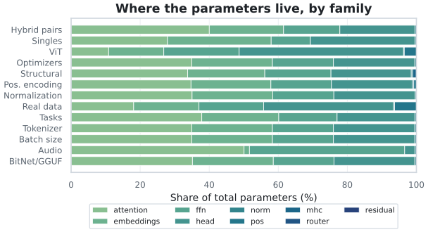
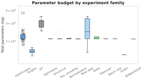
Across the hybrid pairs, the final training loss ranges from 8.116 to
10.450 nats (median 9.595). The best pair is nsa__engram at
8.116, followed by gated_deltanet2__sparda (8.567) and
falcon3__conformer (8.620); the worst,
gqa__tucker, needs 10.450. The spread between the best and
worst pair is wider than the spread between almost all optimizer
ablations—the strongest argument in the round for choosing the attention
pair deliberately: the mixer stack matters more than the optimizer.
Loss and held-out accuracy, however, disagree. Their rank correlation
over the pairs is weak; the pair with the absolute best loss scores 0.0%
top-1, while the best-accuracy pair (fox__falcon1a) reaches
12.55% with a worse training loss (9.292). The reason is resolution:
with four evaluation sentences, a single lucky or unlucky token rewrites
the ranking. Both signals are therefore reported throughout, and the
inference tables should be read as a catastrophic-failure check rather
than as a leaderboard. Table 16 lists
the ten best pairs by final loss and Table 17 the ten
best by held-out accuracy; the two tables have no pair in common.
| Pair (A + B) | Params | Final loss | Top-1 | Top-5 | Train (min) |
|---|---|---|---|---|---|
nsa + engram |
383,999 | 8.116 | 0.00% | 25.0% | 154.5 |
gated_deltanet2 + sparda |
254,336 | 8.567 | 0.00% | 25.0% | 78.2 |
falcon3 + conformer |
254,640 | 8.620 | 4.67% | 25.0% | 32.6 |
falcon1a + conformer |
254,640 | 8.633 | 2.38% | 25.0% | 23.0 |
falcon1 + conformer |
254,640 | 8.639 | 4.67% | 25.0% | 21.3 |
fox + falcon2a |
222,768 | 8.666 | 2.40% | 25.0% | 84.2 |
gqa + conformer |
242,720 | 8.670 | 5.87% | 25.0% | 88.3 |
falcon3a + conformer |
254,640 | 8.681 | 3.97% | 25.0% | 23.2 |
fox + falcon2 |
222,768 | 8.705 | 2.40% | 25.0% | 85.8 |
gla + engram |
387,296 | 8.736 | 5.17% | 25.0% | 149.2 |
| Pair (A + B) | Params | Final loss | Top-1 | Top-5 | Train (min) |
|---|---|---|---|---|---|
fox + falcon1a |
214,232 | 9.292 | 12.55% | 0.0% | 79.3 |
fox + falcon3 |
214,232 | 9.618 | 12.55% | 0.0% | 106.1 |
fox + falcon3a |
214,232 | 9.235 | 12.55% | 0.0% | 77.3 |
gated_deltanet2 + falcon2 |
250,216 | 9.105 | 12.41% | 0.0% | 80.7 |
gated_deltanet2 + falcon2a |
250,216 | 8.968 | 12.41% | 0.0% | 82.1 |
hgrn2 + gated_softmax |
238,688 | 9.386 | 12.30% | 25.0% | 71.7 |
hgrn2 + tucker |
238,688 | 9.221 | 12.30% | 25.0% | 81.6 |
gqla + mlra |
194,624 | 9.461 | 11.85% | 0.0% | 56.0 |
mla + mlra |
194,624 | 9.464 | 11.85% | 0.0% | 86.6 |
deltanet + kda |
231,304 | 9.024 | 11.37% | 0.0% | 78.6 |
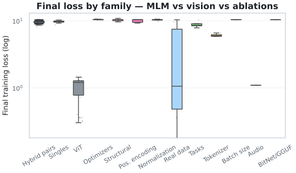
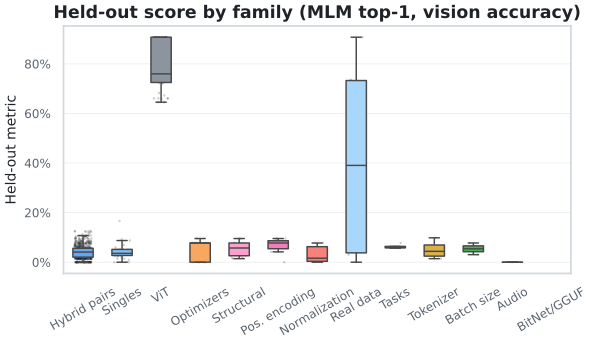
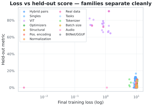
Every run uses the same warm-up-plus-cosine schedule, so the learning curves are directly comparable without re-normalisation. The pair population is still descending at epoch 100: the median loss falls from about 10.2 nats at epoch 0 to 9.49 at the end. The sweep therefore measures speed of learning, not converged quality, and every ranking in this annex should be read as “which pair learns fastest in 3,000 steps” rather than “which pair is best in the limit”.
The optimisation statistics are calm. Gradient norms are stable across families (1.87 for the attention block, 0.92 for the FFN, 3.47 for the head), and the median clip ratio sits at 0.90—below the clipping threshold of 1.0—so most steps pass unclipped and clipping only fires on spikes. The throughput median is 357 tokens/s for the pair population; the 3k–31k tail visible in the charts belongs to the tokenizer and audio ablations, whose step timer covers only part of the work, which is why the Pareto analysis excludes it.
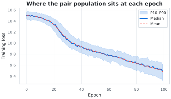
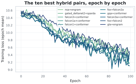
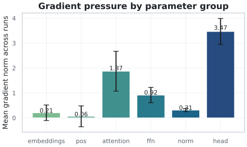
The atlas (Figure 123)
is the centrepiece of the experiment: a matrix in which each cell is one
hybrid pair, rows index the first mixer, columns index the second, and
colour encodes the final loss. It is read in two directions. Column by
column—fix the second mixer, vary the first—the second mixer dominates:
a good B (sparsek, engram, mlra)
keeps almost every A in the 8.9–9.6 nat band, while a bad B
(mamba, retnet, bigbird) drags
even the best A above 10 nats. Row by row—fix the first mixer, vary the
second—no A rescues a bad B. The asymmetry is the visual form of the
first finding of Section 9.
Coverage is almost complete: 667 of the 861 possible pairs were
trained. The 158 pairs that never trained are exactly those containing
cca, ccgqa, msa or
ssog—four mixers that fail in every configuration—which
accounts for the count: \(4\times41 -
\binom{4}{2} = 158\).
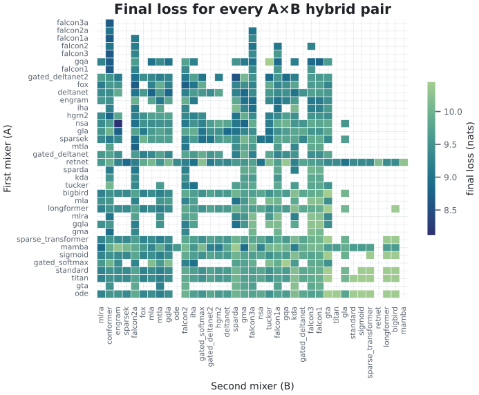
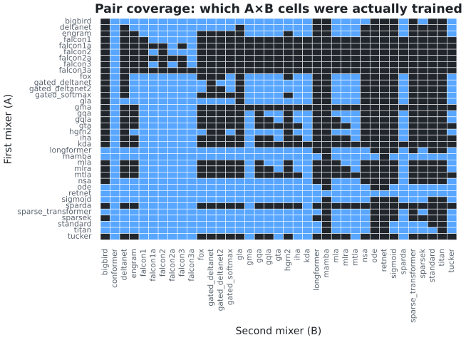
Table 18 ranks second mixers by mean final
loss across every pair that contains them. The Pairs column is
the sample size behind each mean and should be read alongside it: a
single-pair mean (for example mamba, with one pair) is
anecdotal, while a 30–40 pair mean is a solid estimate. The bottom half
of the table is as informative as the top: mamba,
bigbird, longformer and retnet
are cheap but consistently drag their pairs down—exactly the pattern the
heatmaps show, and a warning against equating parameter economy with
quality.
| Second mixer | Pairs | Mean loss | Mean top-1 | Mean params |
|---|---|---|---|---|
mlra |
22 | 9.368 | 5.74% | 209,581 |
conformer |
36 | 9.369 | 3.39% | 259,861 |
engram |
18 | 9.373 | 2.05% | 379,284 |
sparsek |
9 | 9.382 | 4.82% | 208,926 |
falcon2a |
34 | 9.387 | 4.33% | 229,973 |
fox |
16 | 9.409 | 2.23% | 216,038 |
mla |
20 | 9.457 | 4.66% | 217,989 |
mtla |
26 | 9.459 | 5.29% | 217,223 |
falcon1 |
30 | 9.779 | 3.27% | 221,856 |
gta |
25 | 9.788 | 3.27% | 219,828 |
titan |
3 | 9.814 | 6.28% | 204,768 |
gla |
11 | 9.814 | 3.90% | 222,555 |
standard |
4 | 9.960 | 6.65% | 206,264 |
sigmoid |
5 | 10.045 | 4.37% | 207,162 |
sparse_transformer |
6 | 10.108 | 5.59% | 207,760 |
mamba |
1 | 10.279 | 2.04% | 192,608 |
Ranking mixers individually cannot reconstruct the atlas, because
pairs interact. The synergy chart quantifies this: for each pair it
measures how much better (or worse) the pair is than the average of its
two marginal means, \[S_{A,B} = \frac{\mu_A +
\mu_B}{2} - L_{A,B},\] where \(\mu_A\) and \(\mu_B\) are the mean losses of all pairs
containing A and B respectively. Positive synergy means the pair beats
what its parts would predict. nsa+engram gains 1.304 nats,
and the top of the table shares a pattern: a cheap, clean first mixer
stacked under a memory-heavy second one. The negative tail is dominated
by gta, gqa and tucker as
B—mixers that look average in isolation but clash when stacked after a
strong A. For synthesis purposes the message is that a ranked list of
mixers is a necessary summary but an insufficient design tool: the
atlas, or at least the synergy table, must be consulted before composing
a stack.
| Pair | Pair loss | Expected | Synergy | Top-1 |
|---|---|---|---|---|
nsa + engram |
8.116 | 9.420 | \(+1.304\) | 0.00% |
gated_deltanet2 + sparda |
8.567 | 9.448 | \(+0.881\) | 0.00% |
fox + falcon2 |
8.705 | 9.446 | \(+0.741\) | 2.40% |
gqa + falcon1 |
8.784 | 9.518 | \(+0.734\) | 2.86% |
fox + falcon2a |
8.666 | 9.390 | \(+0.724\) | 2.40% |
bigbird + gta |
10.445 | 9.725 | \(-0.720\) | 1.79% |
retnet + gated_softmax |
10.239 | 9.533 | \(-0.706\) | 7.70% |
mamba + engram |
10.277 | 9.543 | \(-0.734\) | 1.10% |
mamba + sparda |
10.391 | 9.643 | \(-0.749\) | 5.09% |
gqa + tucker |
10.450 | 9.432 | \(-1.018\) | 7.76% |
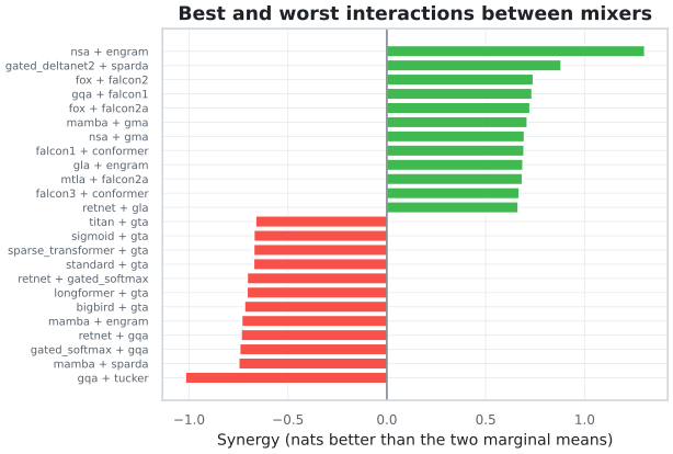
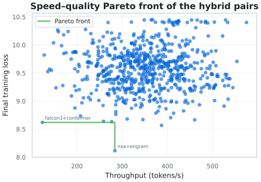
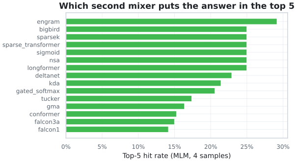
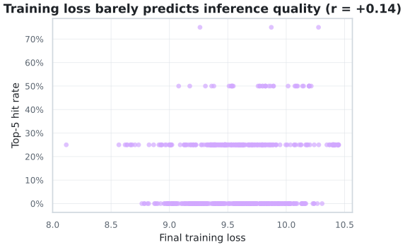
The optimizer sweep is the most sobering chart of the round: 23
optimizers, the same 210k backbone, and a final-loss range of only
10.10–10.77 nats (Table 20).
q_apollo wins at 10.098 and galore_adamw
closes the table at 10.772, but a dozen optimizers land on exactly
10.404—the run is too short for the choice of optimizer to separate from
noise, and the honest summary at this budget is that most modern
optimizers are interchangeable. The speed differences are real, however:
mean step time varies by roughly 30%, and the second-order and
orthogonalised methods (shampoo, muon) pay a
visible overhead. When runs are short, the optimizer is best chosen for
speed rather than for final loss.
| Optimizer | Final loss | Top-1 | Tok/s |
|---|---|---|---|
q_apollo |
10.098 | 3.63% | 436 |
sophia |
10.104 | 1.79% | 378 |
lion |
10.245 | 4.64% | 279 |
shampoo |
10.401 | 7.76% | 382 |
adopt |
10.404 | 7.76% | 391 |
mars_adamw |
10.404 | 7.76% | 343 |
adan |
10.404 | 7.76% | 359 |
adamw |
10.404 | 7.76% | 384 |
schedulefree_adamw |
10.404 | 7.76% | 487 |
soap |
10.404 | 7.76% | 412 |
ademamix |
10.404 | 7.76% | 366 |
cautious_adamw |
10.404 | 7.76% | 365 |
prodigy |
10.439 | 0.00% | 349 |
sgd_momentum |
10.450 | 0.00% | 347 |
turbo_muon |
10.454 | 0.00% | 536 |
anon |
10.458 | 0.00% | 387 |
muon |
10.461 | 0.00% | 507 |
apollo |
10.519 | 0.00% | 401 |
adafactor |
10.530 | 0.00% | 395 |
ada_muon |
10.620 | 1.79% | 497 |
lamb |
10.653 | 7.76% | 464 |
radam |
10.738 | 7.76% | 502 |
galore_adamw |
10.772 | 9.54% | 451 |
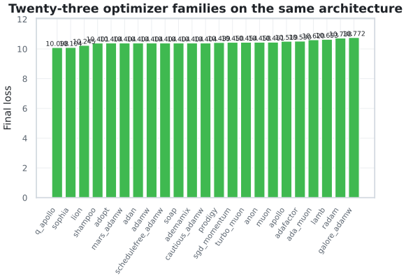
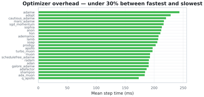
Among the normalizations (Table 21),
flash_norm wins clearly at 9.749 nats—half a nat ahead of
the runner-up, a large margin by the standards of this round—while
prms_norm and rms_norm lag. In the positional
encodings (Table 22), the PAPE family
(pape_ri, pape, pape_efficient)
sweeps the podium, and classical RoPE is mid-table. Both results are
useful calibration: “modern” is not automatically better on a 100-epoch
run at this scale, and component choices that look like refinements in
the literature can separate by half a nat here.
| Variant | Final loss | Top-1 | Params |
|---|---|---|---|
flash_norm |
9.749 | 1.43% | 209,600 |
dynamic_tanh |
10.246 | 0.00% | 210,752 |
derf |
10.295 | 1.79% | 210,762 |
layer_norm |
10.401 | 7.76% | 210,752 |
rms_norm |
10.436 | 7.76% | 210,272 |
prms_norm |
10.573 | 0.00% | 210,272 |
| Encoding | Final loss | Top-1 | Params |
|---|---|---|---|
pari |
9.235 | 0.00% | 211,520 |
pape |
9.455 | 4.17% | 216,928 |
pape_efficient |
9.455 | 4.17% | 216,928 |
learned_absolute |
9.525 | 7.02% | 216,896 |
hope |
10.348 | — | 210,752 |
sinusoidal_absolute |
10.364 | 6.68% | 210,752 |
bam |
10.397 | 9.54% | 210,768 |
nope |
10.397 | 9.54% | 210,752 |
none |
10.397 | 9.54% | 210,752 |
rope |
10.401 | 7.76% | 210,752 |
sinusoidal_rotary |
10.401 | 7.76% | 210,752 |
alibi |
10.417 | 7.76% | 210,752 |
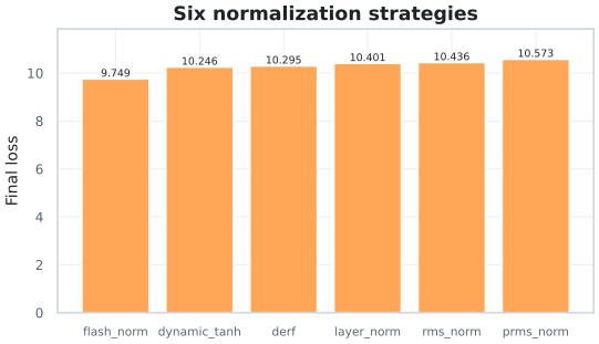
flash_norm separates
from the rest by about half a nat.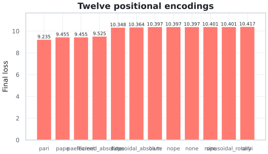
The structural toggles (Table 23) separate more than the optimizers do—evidence that, at this scale, architecture is a stronger lever than the update rule. The three wins are factorised embeddings (9.623), a SwiGLU FFN (9.901) and two Hyperloop loops (9.908). The BitNet toggles land at 10.016, mHC at 10.186, and the residual variants between 10.43 and 10.49. Mixture-of-Depths is the worst switch at 10.854, consistent with its documented incompatibility with mHC at this depth.
| Switch | Final loss | Top-1 | Params |
|---|---|---|---|
factorized_emb |
9.623 | 1.43% | 181,056 |
ffn_swiglu |
9.901 | 2.49% | 228,800 |
num_loops_ |
9.908 | 6.94% | 154,880 |
fixed_softmax_ssmax_bitnet |
9.936 | 2.60% | 209,864 |
bitnet_conv |
10.016 | 2.60% | 209,856 |
bitnet_on |
10.016 | 2.60% | 209,856 |
mhc |
10.186 | 1.79% | 254,092 |
bitnet_routers |
10.327 | — | 247,104 |
ssmax |
10.359 | 9.54% | 210,760 |
ffn_relu |
10.393 | 3.83% | 210,752 |
fixed_both |
10.401 | 7.76% | 210,752 |
embedding_conv |
10.401 | 7.76% | 210,752 |
fixed_ce |
10.401 | 7.76% | 210,752 |
pos_rope |
10.401 | 7.76% | 210,752 |
fixed_softmax |
10.401 | 7.76% | 210,752 |
residuals_full_attn |
10.433 | 9.54% | 210,944 |
residuals_none |
10.476 | 5.71% | 210,752 |
moe |
10.477 | — | 248,384 |
residuals_block_attn |
10.487 | 1.79% | 210,944 |
mod |
10.854 | — | 210,944 |
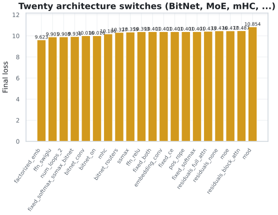
The vision block works. Segmentation reaches 90.7% mean held-out accuracy, classification 75.8% and patch prediction 69.9%. These scores are an order of magnitude above the MLM pairs (4.0% median) because the task is easier, not because the mixer matters more; the report therefore keeps the families separate and draws no cross-family conclusion. The tokenizer and task ablations behave as expected and mainly serve as scale anchors: the tokenizer moves the loss by several nats because it changes the vocabulary and the average sequence length, and the task changes it because the objective itself changes. Neither is comparable with the mixer sweep, and both are excluded from it.
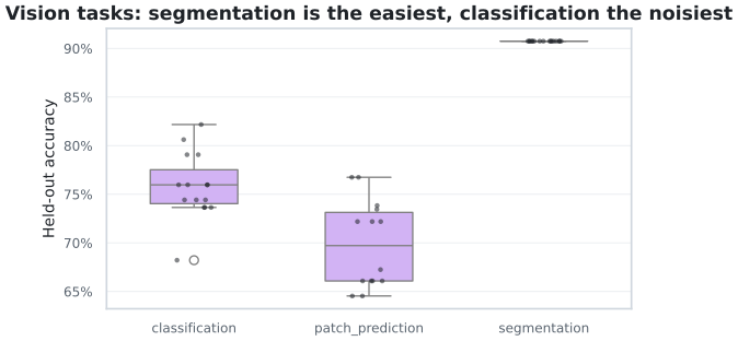
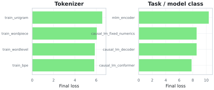
Post-training quantization is the good news of the round. Across the 810 configurations with both formats, mean top-1 moves from 5.62% to 5.43% and mean top-5 from 13.36% to 13.24%—deltas of \(-0.19\) and \(-0.12\) percentage points. Eight hundred of the 810 configurations are exactly unchanged, and the few that move do so by a single sample out of four. For a smoke-scale model this is the expected result, but it is worth measuring rather than assuming.
The speed story is less flattering, and the reason is structural. The quantized deployment is faster than the standard one in only 32.3% of runs (median ratio 0.64\(\times\)) because the deploy stage is dominated by serialisation and format conversion, not by inference; the evaluation stage, which does measure inference, is faster 51.2% of the time with a median 1.03\(\times\) speed-up. Inference itself takes about 10.5 s for four sentences—the number that matters at serving time.
The best inference configuration is not the best-loss configuration.
mamba__engram hits three of four tokens in the top-5
(75.0%) with a training loss of 10.277, above the pair median. With four
samples per configuration, top-5 is a blunt instrument: use it to catch
catastrophic failures, not to crown a winner.
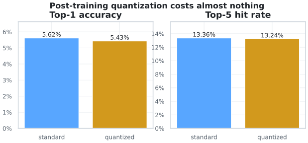
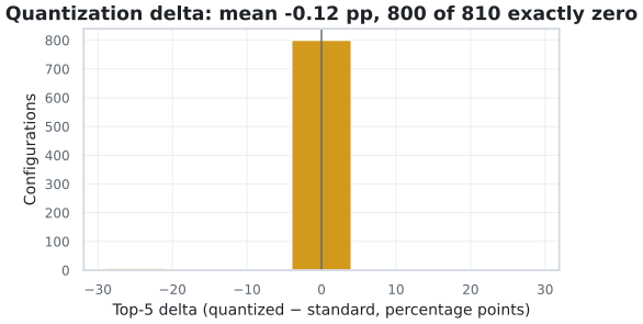
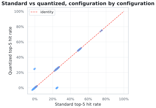
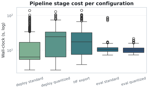
| Configuration | Top-5 std | Top-1 std | Top-5 quant | Final loss | Params |
|---|---|---|---|---|---|
mamba__engram |
75% | 50% | 75% | 10.277 | 347,168 |
mamba__nsa |
75% | 0% | 75% | 9.262 | 192,479 |
retnet__fox |
75% | 0% | 75% | 9.873 | 220,936 |
bigbird__kda |
50% | 0% | 50% | 10.196 | 221,128 |
fox__engram |
50% | 25% | 50% | 9.535 | 375,496 |
fox__gated_softmax |
50% | 25% | 50% | 9.892 | 220,744 |
fox__tucker |
50% | 25% | 50% | 9.890 | 220,744 |
gated_deltanet__tucker |
50% | 25% | 50% | 9.796 | 230,928 |
gla__falcon1 |
50% | 0% | 50% | 9.511 | 226,032 |
gla__mlra |
50% | 25% | 50% | 9.538 | 211,808 |
The ledger records 5,271 stage executions. 868 training runs succeeded and 171 failed with a non-zero exit code—all of them outside the 868 analysed configurations, which were selected precisely because they trained. Deployment failed 104 times out of 1,734, always in symmetric pairs: a configuration that fails the standard export also fails the quantized one, which points to a shared root cause (checkpoint or configuration serialisation) rather than to quantization itself.
Two data-quality findings shape the interpretation of the atlas.
First, four mixers never train: cca, ccgqa,
msa and ssog fail in their four singles and in
all 158 pairs that contain them—exactly the 158 missing cells. Second,
four mixers are indistinguishable at a 32-token context:
standard, bigbird, longformer and
titan share bit-identical losses and parameter counts
because their windows (at least 64 tokens) cover the whole sequence and
the position-augmented variant reduces to plain multi-head attention;
they agree on all 33 shared second mixers. Separately, 37 pairs appear
as attn_retnet__X and attn_retnet__X with
identical metrics—two names for one implementation—which the atlas
collapses to one row. Each of these facts is a caveat carried forward
rather than a defect hidden: the atlas has 667 measured cells, 158
structurally missing ones, and four mixers that are, at this context
length, the same model.
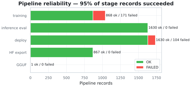
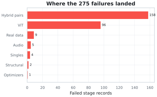
Over the hybrid pairs, parameter count correlates with final loss at \(r = -0.20\) and with held-out accuracy at \(r = -0.07\): size barely buys quality here. What it does predict reliably is cost (\(r = 0.68\) with step time, \(r = 0.65\) with wall-clock). Training loss carries only a weak signal about inference quality (\(r = 0.14\) with top-5)—the quantitative form of the loss/accuracy disagreement noted above. Gradient norm and clip ratio are exactly redundant with each other (\(r = 1.00\)), which is expected because the clip ratio is computed from the gradient norm, and neither correlates with quality.
The correlation matrix of Figure 142 is computed over all 868 rows. Read that way, parameter count correlates with loss at \(-0.43\) and with accuracy at \(+0.42\), apparently contradicting the pair-only numbers. Both readings are correct, and the reconciliation is a textbook confound: the all-rows matrix is dominated by the contrast between vision transformers (larger, much lower loss, much higher accuracy) and MLM pairs, so it measures the gap between families rather than the effect of size within a family. Within the population the atlas is about—the hybrid pairs—size is close to irrelevant, and that is the number to quote.
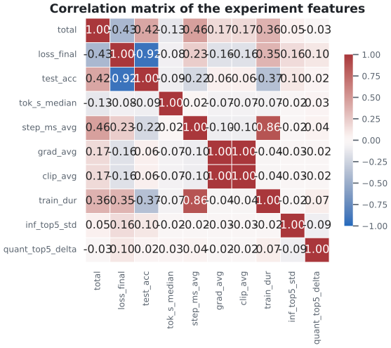
If a pair must be chosen blind, the round supports a simple
heuristic: pick a memory-heavy second mixer (engram,
sparsek, mlra) and a cheap, stable first mixer
(fox, gqa, gated_deltanet2), and
avoid mamba, retnet and bigbird
as B. Expect about \(\pm0.3\) nats of
interaction noise—larger than the difference between most optimizers,
and therefore the dominant uncertainty when composing a stack.
The round also defines its own successor, and its limitations are the
specification. The atlas should be re-run at 256–512 tokens, where the
four window-collapsing mixers become distinguishable and the sparse
patterns actually sparsify; the evaluation should use a 200-sentence
held-out set scored by per-token log-likelihood, because four sentences
cannot rank 800 configurations; the top pairs should train to 300
epochs, because every curve is still descending; the retnet
alias and the four failing mixers should be fixed or removed from the
list; and the ablation families should run at least three seeds, because
their current spread is within seed noise. Finally, quantization should
become the default deployment format: it cost 0.12 points of top-5 and
sped up evaluation in half the runs.
The Frankenstein Transformer toolkit enforces a strict YAML
configuration schema with additionalProperties: false at
all levels. The schema is defined in , which references modular
sub-schemas in . Every configurable field must be declared in the
schema; unrecognized keys are rejected at validation time. This appendix
documents the complete schema structure, including all fields, their
types, constraints, and cross-component validation rules.
The root schema object has the following top-level properties. All
are optional except training, which is required:
base_model (string) — HuggingFace model identifier
or local path for continual pretraining or SBERT fine-tuning. When set,
model_class and model are not required (the
architecture is inferred from the checkpoint).
tokenizer (object) — Tokenizer configuration,
available to both the base_model path and custom
from-scratch models. Two modes are selected via source:
hf_repo (default) loads a pretrained tokenizer from
name_or_path; train_from_dataset trains a new
tokenizer from the dataset text (see §37.4). Required when using
base_model with the mlm task.
model_class (enum) — Model architecture variant:
frankenstein_text_encoder (mixed-architecture encoder),
frankenstein_text_decoder (autoregressive causal decoder),
or frankenstein_vit (vision transformer). Required when
base_model is not set.
model (object) — Model architecture parameters (see
§37.2). Required when
base_model is not set.
training (object, required) —
Training configuration (see §37.3).
The schema enforces a mutual-exclusivity rule: either
base_model must be present, or both
model_class and model must be present.
The model object defines all architectural
hyperparameters. Required fields are dims.vocab_size,
dims.hidden_size, dims.num_layers,
dims.num_heads, and dims.layer_pattern.
Table 25 lists all model fields with
their types and descriptions.
| Field | Type | Description |
|---|---|---|
| Field | Type | Description |
| dims.mode | enum (encoder, decoder) | Attention masking mode.
encoder = bidirectional; decoder =
causal. |
| dims.vocab_size | int \(\ge 1\) (required) | Number of unique tokens in the vocabulary. Must match the tokenizer’s vocab size. |
| dims.hidden_size | int \(\ge 1\) (required) | Hidden dimension. Must be divisible by
num_heads. Typical: 512–2048. |
| dims.num_layers | int \(\ge 1\) (required) | Number of physical transformer layers. Typical: 6–24. |
| dims.num_loops | int \(\ge 1\) | Logical loop count. Each layer in
layer_pattern runs num_loops times. Default:
1. |
| dims.num_heads | int \(\ge 1\) (required) | Number of parallel attention heads. Must
divide hidden_size evenly. |
| dims.dropout | float [0,1] | Global dropout rate. Typical: 0.1 (BERT standard). |
| dims.layer_pattern | array of enum (required) | Ordered sequence of layer types. Length
must equal num_layers. 48 mixer codes available (see
Table 37.2.1). |
| norm.type | enum | Normalization strategy:
layer_norm, dynamic_tanh, derf,
rms_norm, prms_norm,
flash_norm. |
| norm.partial_ratio | float (0,1] | Fraction of hidden dims for pRMSNorm estimation. Default: 0.0625. |
| embedding.factorized.enabled | bool | Enable embedding matrix factorization to reduce parameters. |
| embedding.factorized.dim | int \(\ge 1\) | Intermediate dimension for factorized embeddings. Typical: 64–256. |
| embedding.conv.enabled | bool | Apply Conv1d over token embeddings to capture local n-gram patterns. |
| embedding.conv.kernel | int \(\ge 1\) | Kernel size for embedding Conv1d. Typical: 3. |
| attention.ode.solver | enum (rk4, euler) | Numerical integration method for ODE layers. Default: rk4. |
| attention.ode.steps | int \(\ge 1\) | Integration steps between consecutive transformer layers. Default: 2. |
| attention.retnet.heads | int \(\ge 1\) | Retention heads for retnet
layers. Must divide hidden_size. Default: 8. |
| attention.mla.latent_rank | int \(\ge 1\) | Rank of joint KV latent for MLA. Default:
hidden_size // 2. |
| attention.gqla.latent_rank | int \(\ge 1\) | Rank of joint KV latent for GQLA. Default:
hidden_size // 2. |
| attention.gqla.num_groups | int \(\ge 1\) | Number of GQA groups for GQLA decode path.
Must divide num_heads. |
| attention.gqla.decode_path | enum (mqa_absorb, gqa) | Decoding path for GQLA. |
| attention.mlra.latent_rank | int \(\ge 1\) | Total latent rank for MLRA. Default:
hidden_size // 2. |
| attention.mlra.num_latent_heads | int \(\ge 1\) | Number of disjoint latent sub-spaces for MLRA. Default: 4. |
| attention.tucker.query_rank | int \(\ge 1\) | Tucker rank for query weight tensor.
Default: hidden_size. |
| attention.tucker.key_rank | int \(\ge 1\) | Tucker rank for key weight tensor.
Default: hidden_size // 2. |
| attention.tucker.value_rank | int \(\ge 1\) | Tucker rank for value weight tensor.
Default: hidden_size // 2. |
| attention.kpa.h1 | int \(\ge
1\) (or null) |
Head-partition factor count; \(h_1 h_2 = \texttt{num\_\allowbreak\allowbreak
heads}\). Default: largest proper divisor of
num_heads. |
| attention.kpa.h2 | int \(\ge
1\) (or null) |
Within-head factor count. Default:
num_heads // h1. |
| attention.kpa.d1 | int \(\ge 1\) | Head-partition factor width; \(d_1 d_2 = \texttt{head\_\allowbreak\allowbreak
dim}\). Default: 8 (falls back to the largest divisor of
head_dim). |
| attention.kpa.d2 | int \(\ge
1\) (or null) |
Within-head factor width. Default:
head_dim // d1. |
| attention.kpa.query_rank | int \(\ge 1\) | Number of Kronecker terms for the query. Default: 6. |
| attention.kpa.key_rank | int \(\ge 1\) | Number of Kronecker terms for the key (cached). Default: 2. |
| attention.kpa.value_rank | int \(\ge 1\) | Number of Kronecker terms for the value (cached). Default: 2. |
| attention.tpa.query_rank | int \(\ge 1\) | CP rank \(R_Q\) of the query factors (never cached). Default: 8. |
| attention.tpa.key_rank | int \(\ge 1\) | CP rank \(R_K\) of the key factors (cached). Default: 2. |
| attention.tpa.value_rank | int \(\ge 1\) | CP rank \(R_V\) of the value factors (cached). Default: 2. |
| attention.mfa.factor_rank | int \(\ge 1\) | Low-rank factorization dimension \(C\), equal to the per-head width, the shared \(S_q/S_k/S_v\) width and the per-token KV-cache width. Default: 128. |
| attention.mfa.key_reuse | bool | Enable MFA-KR: \(S_v=(I+\mathrm{diag}(\alpha)N)S_k\) with zero-initialised \(\alpha\); decode caches keys only (\(C\) floats/token). Default: false. |
| attention.iha.num_pseudo_heads | int \(\ge 1\) | Number of pseudo-heads per head for IHA.
Default: num_heads. |
| attention.gta.num_shared_groups | int \(\ge 1\) | Number of head groups sharing an attention
map for GTA. Must divide num_heads. |
| attention.gta.value_latent_rank | int \(\ge 1\) | Rank of value-cache latent for GTA.
Default: hidden_size // 2. |
| attention.mtla.latent_rank | int \(\ge 1\) | Latent rank for MTLA. Default:
hidden_size // 2. |
| attention.mtla.merge_factor | int \(\ge 1\) | Number of consecutive KV entries merged per temporal slot. Default: 2. |
| attention.mtla.stride | int \(\ge 1\) | Stride between merged temporal slots.
Default: mtla_merge_factor. |
| attention.cca.latent_rank | int \(\ge 1\) | Latent width for CCA. Default:
hidden_size // 4. Must be divisible by
num_heads. |
| attention.cca.num_conv_layers | enum (0, 1, 2) | Number of convolution layers in CCA. Default: 2. |
| attention.cca.conv_kernel_seq | int \(\ge 1\) | Kernel size of depth-wise causal sequence conv. Default: 4. |
| attention.cca.conv_kernel_ch | int \(\ge 1\) | Kernel size of head-wise grouped channel conv. Default: 3. |
| attention.cca.qk_mean | bool | Enable q-k-mean bias in CCA. Default:
true. |
| attention.cca.value_shift | bool | Enable value-shift in CCA. Default:
true. |
| attention.ccgqa.query_latent_rank | int \(\ge 1\) | Query latent width for CCGQA. Default:
hidden_size // 2. |
| attention.ccgqa.kv_latent_rank | int \(\ge 1\) | KV latent width for CCGQA. Default:
hidden_size // 8. |
| attention.ccgqa.num_kv_heads | int \(\ge 1\) | Number of KV heads for CCGQA. Must divide
num_heads. |
| attention.ccgqa.num_conv_layers | enum (0, 1, 2) | Number of convolution layers in CCGQA. Default: 2. |
| attention.ccgqa.conv_kernel_seq | int \(\ge 1\) | Kernel size of depth-wise causal sequence conv. Default: 4. |
| attention.ccgqa.conv_kernel_ch | int \(\ge 1\) | Kernel size of head-wise grouped channel conv. Default: 3. |
| attention.ccgqa.qk_mean | bool | Enable q-k-mean bias in CCGQA. Default:
true. |
| attention.ccgqa.value_shift | bool | Enable value-shift in CCGQA. Default:
true. |
| attention.msa.block_size | int \(\ge 1\) | Block size for MiniMax Sparse Attention. Default: 128. |
| attention.msa.topk_blocks | int \(\ge 1\) | Number of blocks selected per GQA group per query. Default: 16. |
| attention.msa.index_dim | int \(\ge 1\) | Dimensionality of Index Branch heads. Default: 64. |
| attention.msa.kl_loss_weight | float \(\ge 0\) | Weight of KL alignment loss for MSA index branch. Default: 0.0. |
| attention.sparda.block_size | int \(\ge 1\) | KV block size for SparDA. Default: 128. |
| attention.sparda.topk_blocks | int \(\ge 1\) | Number of KV blocks selected per GQA group. Default: 16. |
| attention.sparda.forecast_dim | int \(\ge 1\) | Dimensionality of Forecast projection. Default: 64. |
| attention.lsa.num_long_range | int \(\ge 1\) | Long-range key budget \(k\) selected per query. Default: 2048. |
| attention.lsa.num_buckets | int \(\ge 1\) | Buckets scored per query \(p\); raised so \(p\cdot\)pool_size \(\ge k\). Default: 512. |
| attention.lsa.num_sinks | int \(\ge 1\) | Always-attended leading sink keys. Default: 4. |
| attention.lsa.pool_size | int \(\ge 1\) | Keys summed per pool key before Ward clustering. Default: 4. |
| attention.lsa.cluster_block | int \(\ge 2\) | Cluster block size; also the window \(n_w\). Default: 512. |
| attention.lsa.keys_per_bucket | int \(\ge 1\) | Average keys per bucket; yields
cluster_block / keys_per_bucket buckets per block. Default:
8. |
| attention.lsa.max_keys_per_bucket | int \(\ge 1\) | Merge cap per bucket. Default: 16. |
| attention.fastconformer.window_size | int \(\ge 2\) | Total local span \(w\); per-side context \(w/2\) (paper: 128 each side). Default: 256. |
| attention.fastconformer.global_tokens | int \(\ge 0\) | Leading global attention tokens \(g\) (paper: 1; 0 = pure limited context). Default: 1. |
| attention.fastconformer.global_tokens_spacing | int \(\ge 1\) | Stride \(s\) between global positions \(\{0, s, \dots, (g{-}1)s\}\). Default: 1. |
| attention.fastconformer.global_attn_separate | bool | Separate global Q/K/V projections (\(+3H^2\); §2.2) vs shared (§3.4). Default: false. |
| attention.engram.max_ngram_size | int \(\ge 2\) | Maximum N-gram order for Engram memory module. |
| attention.engram.n_heads_per_ngram | int \(\ge 1\) | Number of hash heads per N-gram order. |
| attention.engram.embed_dim_per_head | int \(\ge 1\) | Embedding dimension per hash head. |
| attention.engram.kernel_size | int \(\ge 1\) | Causal depthwise conv kernel width for Engram. |
| attention.engram.seed | int | Random seed for N-gram hash multipliers. |
| mhc.enabled | bool | Enable the manifold-constrained n-stream
residual (mHC, arXiv:2512.24880). Default: false. |
| mhc.expansion_rate | int \(\ge 1\) | Residual-stream expansion factor \(n\). The stream becomes \(n \times\) hidden_size. \(1\) recovers the identity mapping. Default:
4. |
| mhc.sinkhorn_iters | int \(\ge 1\) | Sinkhorn-Knopp normalisation rounds constraining \(H^{\text{res}}\) to be doubly stochastic. Default: 20. |
| mhc.gating_init | float \(> 0\) | Initial value of the mHC gating scalars \(\alpha\). Default: 0.01. |
| mhc.checkpoint | bool | Gradient checkpointing on mHC layers to
mitigate the \(\sim n\times\)
activation-memory increase. Default: false. |
| mhc.full_prec_under_bitnet | bool | Keep the mHC coefficient projection
full-precision under BitNet. Default: true. |
| moe.enabled | bool | Enable Mixture of Experts in FFN layers.
Default: true. |
| moe.num_experts | int \(\ge 1\) | Total number of expert networks. Default: 8. |
| moe.top_k | int \(\ge 1\) | Experts activated per token. Must be \(\le\) num_experts. Default:
2. |
| bitnet.enabled | bool | Enable BitLinear ternary weight
quantization. Default: true. |
| bitnet.routers | bool | Also quantize routing/scoring projections.
Requires bitnet.enabled=true. Default:
false. |
| bitnet.conv | bool | Quantize embedding Conv1d with BitConv1d.
Requires bitnet.enabled=true and
embedding.conv.enabled=true. Default:
false. |
| mixture_of_depths.enabled | bool | Enable Mixture-of-Depths token routing.
Default: false. |
| mixture_of_depths.capacity_ratio | float (0,1] | Fraction of tokens updated per layer. Default: 0.5. |
| mixture_of_depths.router_aux_loss_weight | float \(\ge 0\) | Weight for the router auxiliary loss. Default: 0.0. |
| ssmax.enabled | bool | Enable Scalable Softmax
(arXiv:2505.22842). Default: false. |
| ssmax.s_init | float \(> 0\) | Initial per-head SSMax scalar. Default: 1.0. |
| numerics.fixed_softmax | bool | Cancellation-free softmax/log-softmax
(arXiv:2610.31642). Default: false. |
| numerics.fixed_cross_entropy | bool | Hard-target CE with zero-sum gradient by
construction (arXiv:2610.31642). Default: false. |
| ffn.hidden_size | int \(\ge 1\) | Intermediate FFN dimension. Default: \(2\times\) hidden_size. |
| ffn.activation | enum | FFN non-linearity (43 values). Default:
silu. |
| ffn.activation_config | object | Parameters for learnable/parametric activations. |
| classification_head.enabled | bool | Enable the NLP sequence-classification
head. Default: false. |
| classification_head.num_labels | int or null | Number of classes. |
| classification_head.pooling_mode | enum (cls, gap) | Pooling for the classification head.
Default: cls. |
Fields are grouped under hierarchical sub-objects (dims,
norm, embedding, attention,
moe, bitnet, mixture_of_depths,
ssmax, numerics, ffn,
classification_head, mhc,
residuals); each sub-header row marks the prefix in effect
for the rows that follow it. There are no flat feature keys at
model.*.
The model.dims.layer_pattern array accepts the following
48 mixer codes. Each element defines one physical layer in the model
stack. Table 26 lists all available types
with their training and inference support.
| Type | Description | Train | Infer |
|---|---|---|---|
| Type | Description | Train | Infer |
| standard | Classic multi-head self-attention (BERT-style) | ||
| sigmoid | Sigmoid-gated attention | ||
| ca | Continuum Attention — exact continuous integration over piecewise-linear memory trajectories | ||
| xsa | Exclusive Self Attention — post-SDPA orthogonalization against the self value vector | ||
| mta | Multi-Token Attention — causal key-query and head-group convolutions over the attention score map with a gated group norm | ||
| memory | Memory Attention — token-ID memory values (V = K + Norm(E[s])) | ||
| gated_softmax | Gated softmax attention with post-SDPA sigmoid | ||
| titan | Titan attention with positional encoding (HoPE/RoPE) | ||
| retnet | Retention Network (RNN+transformer hybrid) | ||
| mamba | Selective state-space model (SSM) | ||
| ode | Continuous-depth ODE layer | ||
| gla | Gated Linear Attention with multiplicative decay | ||
| deltanet / gated_deltanet | DeltaNet with corrective delta rule | ||
| gated_deltanet2 | Gated DeltaNet-2 with decoupled channel-wise erase/write gates | ||
| hgrn2 | HGRN2 with hierarchical forget gates | ||
| fox | Forgetting Transformer (FoX) with forget bias in logits | ||
| fpa | First Passage Attention with a range-minimum forget bias | ||
| nsa | Native Sparse Attention (three-branch) | ||
| engram | N-gram conditional memory lookup | ||
| gqa | Grouped-Query Attention with configurable KV heads | ||
| longformer | Longformer: sliding windows + global tokens | ||
| bigbird | BigBird: local + random + global attention | ||
| sparse_transformer | Sparse Transformer: factorized patterns | ||
| sparsek | SparseK: differentiable top-k KV selection | ||
| probsparse | ProbSparse: query-sparsity top-u selection with relative-position terms | ||
| sparge | SpargeAttn — two-stage block pruning; dense training, sparse inference | ||
| fasa | FASA — frequency-aware token selection; dense training, sparse inference | ||
| msa | MiniMax Sparse Attention — block-sparse on GQA | ||
| sparda | SparDA — decoupled sparse attention with Forecast projection | ||
| lsa | Latent Sparse Attention — semantic key clustering with top-k selection | ||
| fastconformer | Fast Conformer — limited-context window + head-pinned global token | ||
| kda | Kimi Delta Attention — channel-wise decay + scalar write gate | ||
| falcon1 / falcon2 / falcon3 | Falcon regression family — RAW prefix-aligned NLMS delta rule | ||
| falcon1a / falcon2a / falcon3a | Falcon inner-product family — shifted additive writes with ridge decay | ||
| mla | Multi-Head Latent Attention + RoPE | ||
| gqla | Group-Query Latent Attention — two decoding paths | ||
| mlra | Multi-Head Low-Rank Attention — partitionable latent | ||
| tucker | Tucker Attention — generalised low-rank factorisation | ||
| kpa | Kronecker Product Attention — Kronecker-sum K/V factors, Kronecker-Separable RoPE | ||
| tpa | Tensor Product Attention — CP vector-factor Q/K/V, factorized KV cache, RoPE-compatible | ||
| mfa | Multi-matrix Factorization Attention — shared low-rank QK, single shared K/V head, MFA-KR key reuse | ||
| iha | Interleaved Head Attention — cross-head pseudo-heads | ||
| gta | Grouped-head laTenT Attention — shared map + latent values | ||
| mtla | Multi-head Temporal Latent Attention — temporal KV merge | ||
| cca | Compressed Convolutional Attention — latent-space attention + convs | ||
| ccgqa | Compressed Convolutional Grouped Query Attention — CCA + GQA in latent | ||
| gma | Gaussian Mixture Attention — probabilistic latent routing, \(\mathcal{O}(NK)\) linear-time | ||
| ssog | Separable Sum of Gaussians — Gaussian field over relative position, near-linear \(\mathcal{O}(R N \sqrt{N})\) |
The training object controls the entire training
pipeline. The only required field is task. Table 27 lists all training
fields.
| Field | Type | Description |
|---|---|---|
| Field | Type | Description |
| task | enum (mlm, sbert, causal_lm) (required) | Training objective. mlm =
Masked Language Modeling; sbert = Sentence-BERT
fine-tuning; causal_lm = autoregressive next-token
prediction (requires
model_class=’frankenstein_text_decoder’). |
| num_epochs | int \(\ge 1\) | Complete passes through the training dataset (MLM only). |
| batch_size | int \(\ge 1\) | Examples per optimizer step (before gradient accumulation). |
| dataloader_workers | int \(\ge 0\) | Parallel worker processes for data loading. |
| max_length | int \(\ge 1\) | Maximum token sequence length. Typical: 128–2048. |
| mlm_probability | float [0,1] | Fraction of tokens masked for MLM prediction. Standard: 0.15. |
| max_samples | int \(\ge 1\) | Total samples before stopping, independent of epochs. |
| test_percentage | float [0,100] | Fraction of the dataset held out from
training and evaluated at the end; the result is written to
test_metrics.json. Default: 0 (disabled). |
| dataset_batch_size | int \(\ge 1\) | Internal batch size for streaming dataset. |
| num_workers | int \(\ge 0\) | Parallel workers for dataset streaming pipeline. |
| cache_dir | string | Directory for caching processed datasets. |
| local_parquet_dir | string | Path to local parquet files for offline streaming. |
| prefer_local_cache | bool | Check local cache first before remote download. |
| stream_local_parquet | bool | Stream from local parquet when
local_parquet_dir is set. |
| join_temp_data_context_window | int \(\ge 0\) | If \(>0\), joins cached token chunks into sequences of this length. |
| join_temp_data_min_remainder_tokens | int \(\ge 0\) | Minimum content tokens in last partial joined window. |
| use_amp | bool | Enable FP16 mixed precision. |
| gradient_accumulation_steps | int \(\ge 1\) | Accumulate gradients over N mini-batches before optimizer step. |
| optimizer | object | Optimizer configuration (see §37.5). Required when
task=mlm or task=causal_lm. |
| sbert | object | SBERT training configuration (see §37.6). Required when
task=sbert. |
| scheduler_total_steps | int \(\ge 1\) | Total optimizer steps for LR schedule. |
| scheduler_warmup_ratio | float [0,1] | Fraction of
scheduler_total_steps for LR warmup. |
| scheduler_type | enum (cosine, constant, linear_warmup_then_constant) | LR decay strategy. |
| grad_clip_max_norm | float \(\ge 0\) | Maximum allowed gradient norm. 0 = disabled. |
| inf_post_clip_threshold | float \(\ge 0\) | Threshold for flagging post-clip gradient explosions. |
| max_nan_retries | int \(\ge 0\) | Maximum retries on NaN/Inf gradients before stopping. |
| checkpoint_every_n_steps | int \(\ge 1\) | Save rolling checkpoint every N steps. |
| max_rolling_checkpoints | int \(\ge 1\) | Maximum rolling checkpoints kept. Oldest deleted when exceeded. |
| num_best_checkpoints | int \(\ge 1\) | Number of best checkpoints kept permanently (by validation loss). |
| nan_check_interval | int \(\ge 1\) | Steps between NaN/Inf checks. |
| log_gradient_stats | bool | Log per-layer gradient norms, min/max. |
| gradient_log_interval | int \(\ge 1\) | Steps between gradient stat logs. |
| csv_log_path | string | File path for step-level training metrics in CSV format. |
| csv_rotate_on_schema_change | bool | Rotate CSV file when schema changes. |
| gpu_metrics_backend | enum (nvml, none) | GPU telemetry backend. |
| nvml_device_index | int \(\ge 0\) | GPU index to monitor (0 = first GPU). |
| enable_block_grad_norms | bool | Log gradient norms per block (embeddings, attention, FFN, etc.). |
| telemetry_log_interval | int \(\ge 1\) | Steps between heavy telemetry logs. |
| gpu_temp_guard_enabled | bool | Strict GPU temperature monitoring.
Requires gpu_metrics_backend=nvml. |
| switch_on_thermal | bool | Critical temp triggers GPU\(\to\)CPU fallback, auto-resume on cooldown. |
| gpu_temp_pause_threshold_c | float | Temperature (\(^\circ\)C) to pause training. |
| gpu_temp_resume_threshold_c | float | Temperature (\(^\circ\)C) to resume training after pause. |
| gpu_temp_critical_threshold_c | float | Informational logging marker for severe thermal events. |
| gpu_temp_poll_interval_seconds | float | Seconds between temp checks during cooldown wait. |
| use_galore | bool | Enable Gradient Low-Rank Projection for memory-efficient training. |
| galore_rank | int \(\ge 1\) | Low-rank projection dimension for GaLore. |
| galore_update_interval | int \(\ge 1\) | Steps between projection matrix recomputation. |
| galore_scale | float \(\ge 0\) | Scaling factor for projected gradients. |
| galore_max_dim | int \(\ge 1\) | Maximum tensor dimension for GaLore projection. |
| hf_output_dir | string | Directory for saving final model via
save_pretrained(). |
The top-level tokenizer object is available to both
training paths: the base_model route (continual pretraining
/ fine-tuning, where the tokenizer must match the pretrained checkpoint)
and the custom from-scratch route (where it resolves the vocabulary
before the embedding matrix is allocated). The source field
selects between two modes:
hf_repo (default) — loads a pretrained tokenizer
from name_or_path (a HuggingFace repo id or local path)
through AutoTokenizer.from_pretrained(). Complementary
flags: use_fast (Rust-backed fast tokenizer, default
true) and trust_remote_code (default
false).
train_from_dataset — trains a new tokenizer
from the corpus text with the HuggingFace tokenizers
library. The corpus is the top-level text_dataset block (HF
hub id, optionally streamed, or a local parquet/json directory); when
the config is driven by an embedding host such as dashAI, the host’s run
dataset can supply it instead. The resulting vocabulary size is injected
into model.dims.vocab_size before model construction, so
the embedding matrix always matches the tokenizer. In this mode
name_or_path must be omitted.
Table 28 lists the
tokenizer.training sub-object fields.
| Field | Type | Description |
|---|---|---|
| Field | Type | Description |
| algorithm | enum (bpe, wordpiece, wordlevel, unigram) | Tokenizer training algorithm.
bpe (Byte Pair Encoding, GPT-2 style, default);
wordpiece (original BERT); wordlevel (word
lookup table); unigram (subword language model,
auto-pruning). |
| vocab_size | int \(\ge 1\) | Target vocabulary size. Required for
bpe/wordpiece/wordlevel; optional
for unigram. |
| min_frequency | int \(\ge 1\) | Minimum token frequency to keep (default 2). |
| special_tokens | array of string | Special tokens registered in the tokenizer
(default [PAD]/[UNK]/[CLS]/[SEP]/[MASK]). |
| save_dir | string | Directory persisted via
save_pretrained(). |
| lowercase | bool | Lowercase all text before training
(default false). |
| strip_accents | bool | Strip diacritics before training (default
false). |
| pre_tokenizer | enum (whitespace, bytelevel, bert) | Pre-tokenization strategy (default
whitespace). |
| max_token_length | int \(\ge 0\) | Per-token character cap; 0 disables the limit. |
The training.optimizer object has two fields:
optimizer_class (enum, required) — One of 23
optimizer algorithms: sgd_momentum, adamw,
adafactor, galore_adamw, prodigy,
lion, sophia, muon,
turbo_muon, radam, adan,
adopt, ademamix, mars_adamw,
cautious_adamw, lamb,
schedulefree_adamw, shampoo,
soap, anon, apollo,
apollo_mini, q_apollo.
parameters (object) — Optimizer hyperparameters with
prefixed keys in the format
<optimizer>-<group>_<param>.
All optimizers support the following per-parameter-group suffixes,
prefixed by the optimizer class name (e.g.,
adamw-lr_embeddings):
Learning rate groups:
lr_embeddings, lr_norms,
lr_attention, lr_other
Weight decay groups: wd_embeddings,
wd_norms, wd_attention,
wd_other
Beta groups: betas_embeddings,
betas_norms, betas_attention,
betas_other
Epsilon groups: eps_embeddings,
eps_norms, eps_attention,
eps_other
Note: parameters of ODE, RetNet, and Mamba mixers are routed into the
attention group rather than having dedicated groups.
Table 29 lists the additional global suffixes supported by each optimizer (prefixed by the optimizer name).
| Optimizer | Specific Global Suffixes |
|---|---|
| Optimizer | Specific Global Suffixes |
| sgd_momentum | momentum,
nesterov |
| adamw | (none — shared suffixes only) |
| adafactor | beta2_decay,
clip_threshold, eps1, eps2 |
| galore_adamw | rank,
update_proj_gap |
| prodigy | d_coef |
| lion | (none — shared suffixes only) |
| sophia | rho,
update_k |
| muon | momentum,
nesterov, ns_steps, ns_eps |
| turbo_muon | momentum,
nesterov, ns_steps, ns_eps |
| radam | (none — shared suffixes only) |
| adan | (none — shared suffixes only) |
| adopt | (none — shared suffixes only) |
| ademamix | (none — shared suffixes only) |
| mars_adamw | (none — shared suffixes only) |
| cautious_adamw | cautious_clip |
| lamb | (none — shared suffixes only) |
| schedulefree_adamw | (none — shared suffixes only) |
| shampoo | (none — shared suffixes only) |
| soap | (none — shared suffixes only) |
| anon | gamma |
| apollo | rank,
update_proj_gap, scale,
scale_type, proj_type,
scale_front, disable_nl |
| apollo_mini | update_proj_gap,
scale, proj_type, scale_front,
disable_nl |
| q_apollo | rank,
update_proj_gap, scale,
scale_type, proj_type,
scale_front, disable_nl,
quant_bits |
The training.sbert object configures Sentence-BERT
fine-tuning. It is required when training.task=sbert. Key
fields include:
dataset_name (string) — HuggingFace dataset ID or
local path.
dataset_type (enum) —
paired_similarity, triplets, or
qa.
columns (object) — Optional column name overrides
for dataset fields.
query_prefix / document_prefix (string)
— Text prepended to query/document fields during tokenization.
output_dir (string) — Directory for SBERT
artifacts.
batch_size (int) — Examples per batch. Typical:
16–64.
gradient_accumulation_steps (int) — Accumulation
steps for SBERT.
grad_clip_max_norm (float) — Gradient clipping
threshold. Typical: 0.5–2.0.
num_epochs (int) — Complete passes through SBERT
dataset. Typical: 1–10.
warmup_steps (int) — Steps for LR warmup.
evaluation_steps (int) — Evaluate every N
steps.
checkpoint_save_steps (int) — Save rolling
checkpoint every N steps.
resume_from_checkpoint (string or null) —
auto resumes from the latest checkpoint; null
starts fresh.
learning_rate (float) — Initial LR. Typical: \(1\times10^{-5}\) to \(1\times10^{-4}\).
max_train_samples / max_eval_samples
(int) — Limit training/evaluation samples.
max_length (int) — Max token length for input texts.
Typical: 128–512.
pooling_mode (enum) — mean,
cls, or max.
trust_remote_code (bool) — Allow custom code from
model repo.
use_amp (bool) — Enable FP16 mixed
precision.
resample_balanced (bool) — Resample to balanced
distribution over similarity scores.
standardize_scores (bool) — Z-score normalize
similarity scores.
resample_std (float) — Target std dev when
standardize_scores=true.
optimizer (object) — Custom optimizer for SBERT
(same classes as MLM training); constructor kwargs go under
optimizer.optimizer_kwargs.
wandb_project (string) — Weights & Biases
project name for telemetry.
The schema enforces the following cross-component validation rules,
implemented both in the JSON Schema
(_conditional_rules.yaml) and at runtime in the
configuration loader:
additionalProperties: false is enforced at all
nesting levels. Any unrecognized key in any object triggers a validation
error.
model.dims.hidden_size must be divisible by
model.dims.num_heads. The per-head dimension is \(\texttt{hidden\_\allowbreak size} /
\texttt{num\_\allowbreak heads}\).
model.dims.num_kv_heads must divide
model.dims.num_heads exactly when Grouped-Query Attention
is used.
vocab_size must match the tokenizer’s vocabulary
size. Mismatch causes token ID corruption and unrecoverable training
failure.
When base_model is set, training.task
is required. If task=mlm,
tokenizer.name_or_path is also required — unless
tokenizer.source=train_from_dataset, in which case the
tokenizer is trained from the corpus and no name is needed.
tokenizer.source=train_from_dataset requires the
tokenizer.training sub-object (with vocab_size
for bpe/wordpiece/wordlevel) and
is mutually exclusive with tokenizer.name_or_path. The
trained vocabulary overrides model.dims.vocab_size before
model construction.
task: mlm requires training.optimizer;
task: sbert requires training.sbert;
task: causal_lm requires training.optimizer
and model_class=’frankenstein_text_decoder’.
bitnet.routers=true requires
bitnet.enabled=true. The flag has no effect
otherwise.
mhc.enabled=true (mHC n-stream residual) and
mixture_of_depths.enabled=true are mutually exclusive.
Enabling both raises a ValueError: MoD token routing
operates on a single \(C\)-dimensional
stream, which conflicts with the n-stream residual.
fasa and sparge are inference-sparse
layer types: they apply their sparse heuristic only in evaluation mode.
During training the enclosing hybrid layer substitutes standard dense
attention over the same \(\mathbf{q}/\mathbf{k}/\mathbf{v}/\mathbf{o}\)
projections, so they can appear in model.dims.layer_pattern
for training runs; the trained weights are the ones the sparse path
reads at inference.
model_class: frankenstein_text_decoder forces
model.dims.mode: decoder at runtime. Setting
model.dims.mode: encoder with this class is
overridden.
Either base_model must be present, or both
model_class and model must be present. The
schema rejects configurations that provide neither or an incomplete
combination.
This appendix provides a complete reference of all components implemented in the Frankenstein Transformer codebase: 56 sequence mixers across nine families, 39 optimizers, 6 normalization variants, 43 activation functions, and 4 embedding methods. Each table is self-contained and cross-references the bibliography.
Table [tab:all-mixers] enumerates every
sequence mixer supported by the layer_pattern schema field,
organized by architectural family. Training and inference complexity are
expressed in terms of sequence length \(n\), hidden dimension \(d\), and family-specific parameters.
L1.9cmL2.0cmL2.4cmL2.4cmL3.3cmL2.3cm
Name & Family &
Training & Inference &
Key Characteristic &
Reference
Name & Family &
Training & Inference &
Key Characteristic &
Reference
standard & Dense & \(\mathcal{O}(n^2
d)\) & \(\mathcal{O}(n)\)
cache & Full global context; KV bottleneck at long sequences &
sigmoid & Dense & \(\mathcal{O}(n^2
d)\) & \(\mathcal{O}(n)\)
cache & Element-wise gating; hardware-efficient replacement for
softmax &
gqa & Dense & \(\mathcal{O}(n^2
d)\) & \(\mathcal{O}(n)\)
cache & Tunable KV compression; \(G\times\) cache reduction via shared heads
&
ca & Dense & \(\mathcal{O}(n^2
d)\) & \(\mathcal{O}(n)\)
cache & Exact integration over piecewise-linear key/value
trajectories; half-token caps; nonnegative normalized effective weights
&
xsa & Dense & \(\mathcal{O}(n^2
d)\) & \(\mathcal{O}(n)\)
cache & Post-SDPA orthogonalization against the self value vector;
zero extra parameters; implicit attention sink &
mta & Dense & \(\mathcal{O}(n^2 (d +
c_q c_k) n_h)\) & \(\mathcal{O}(n)\) cache + query tail &
Key-query (\(c_q\times c_k\)) and
head-group (\(c_h\)) convolutions over
the score map, pre and post softmax; gated group norm; \(+0.001\%\) parameters at 880M &
conformer & Conv-augmented & \(\mathcal{O}(n^2 d + n K d)\) & \(\mathcal{O}(n)\) (full recompute) &
Macaron FFNs around relative-sinusoidal MHSA and a depthwise-conv module
(\(K=32\)); local and global context in
one block &
fastconformer & Conv-augmented & \(\mathcal{O}(n \cdot (w + g) \cdot d)\)
& \(\mathcal{O}(w + g)\) &
Limited-context window + head-pinned global token; optional separate
global projections; linear-memory long-form &
retnet & Recurrent & \(\mathcal{O}(n^2
d)\) parallel & \(\mathcal{O}(1)\) & Multi-scale decay;
triple computation mode (parallel, recurrent, chunkwise) &
mamba & Recurrent & \(\mathcal{O}(n
d)\) & \(\mathcal{O}(1)\)
& Selective state-space model; hardware-aware parallel scan &
ode & Recurrent & \(\mathcal{O}(k
\cdot n^2 d)\) & \(\mathcal{O}(k
n)\) & Continuous-depth RK4 integration; adaptive step solver
&
sparse_transformer & Sparse & \(\mathcal{O}(n \sqrt{n} \cdot d)\) &
\(\mathcal{O}(n)\) & Factorized
strided + fixed masks; \(\sqrt{n}\)
sparsity pattern &
longformer & Sparse & \(\mathcal{O}(n
\cdot w \cdot d)\) & \(\mathcal{O}(n)\) & Sliding window +
dilation + global tokens; linear in \(n\) &
swa & Sparse & \(\mathcal{O}(n \cdot w
\cdot d)\) & \(\mathcal{O}(w)\) & Sliding window +
attention sinks; training-free, fixed KV cache &
bigbird & Sparse & \(\mathcal{O}(n)\) & \(\mathcal{O}(n)\) & Random + local +
global; Turing complete attention &
sparsek & Sparse & \(\mathcal{O}(n
\cdot d)\) & \(\mathcal{O}(k)\) & Differentiable
top-\(k\) selection; learned sparsity
mask &
probsparse & Sparse & \(\mathcal{O}(L
\log L \cdot d)\) & \(\mathcal{O}(n_{\text{ctx}})\) &
Query-sparsity top-\(u\) via max–mean
KL measure; exact KV-cache decode &
nsa & Sparse & \(\mathcal{O}((t/d +
n_l + w)d)\) & \(\mathcal{O}(n)\) & Hardware-aligned
3-branch design; token/neighbor/window &
sparge & Sparse & \(\mathcal{O}(n^2
\cdot s \cdot d)\) & \(\mathcal{O}(n)\) & Two-stage block
filtering; dense training, sparse inference &
fasa & Sparse & \(\mathcal{O}(t \cdot
N_{\text{tip}} + N_{\text{fac}} \cdot d)\) & \(\mathcal{O}(n)\) & RoPE frequency-aware
sparse; dense training, sparse inference &
msa & Sparse & \(\mathcal{O}(H_{\text{kv}} \cdot d_{\text{idx}}
\cdot N^2 + H_q \cdot d_h \cdot N \cdot k \cdot B_k)\) &
\(\mathcal{O}(n)\) & Index-branch
block sparse; deployed at 109B scale &
sparda & Sparse & \(\mathcal{O}(H_{\text{kv}} \cdot d_f \cdot N \cdot
N_b + H_q \cdot d_h \cdot N \cdot k \cdot B_k)\) & \(\mathcal{O}(n)\) & Forecast-guided
lookahead prefetch; predictive sparsity &
lsa & Sparse & \(\mathcal{O}(N^2/\bar{n}_b +
N\,(k+n_w+n_{\text{sink}})\,d_h)\) & \(\mathcal{O}(N/\bar{n}_b +
k+n_w+n_{\text{sink}})\) & Semantic Ward clustering of keys;
top-\(k\) long-range selection;
natively trainable, no extra parameters &
gla & Gated & \(\mathcal{O}(L
d^2)\) & \(\mathcal{O}(d^2)\) & Data-dependent
diagonal decay; linear attention with gating &
deltanet & Gated & \(\mathcal{O}(L
d^2)\) & \(\mathcal{O}(d^2)\) & Delta rule;
error-correcting linear attention &
gated_deltanet & Gated & \(\mathcal{O}(L d^2)\) & \(\mathcal{O}(d^2)\) & Decay + write
gating synthesis; unified delta framework &
gated_deltanet2 & Gated & \(\mathcal{O}(L d^2)\) & \(\mathcal{O}(d^2)\) & Decoupled
channel-wise erase/write; improved gating &
hgrn2 & Gated & \(\mathcal{O}(L
d^2)\) & \(\mathcal{O}(d^2)\) & Hierarchical
bounded forget gates; multi-scale recurrence &
fox & Gated & \(\mathcal{O}(L^2
d)\) & \(\mathcal{O}(L)\) KV
& Logit-space recency bias; FlashAttn compatible &
gated_softmax & Gated & \(\mathcal{O}(L^2 d)\) & \(\mathcal{O}(L)\) KV & Post-SDPA sigmoid
gating; attention-sink mitigation &
kda & Gated & \(\mathcal{O}(L
d^2)\) & \(\mathcal{O}(d^2)\) & Channel-wise decay
+ scalar write; Kimi Linear design &
fpa & Gated & \(\mathcal{O}(L^2
d)\) & \(\mathcal{O}(L)\) KV
& Path-extremum (range-min) forget bias; contains FoX; two extra
scalars per cached key/head &
falcon1 & Fast-weight & \(\mathcal{O}(L d^2)\) & \(\mathcal{O}(d^2)\) & Prefix-aligned
NLMS delta rule; best LM perplexity of the family &
falcon2 & Fast-weight & \(\mathcal{O}(L d^2)\) & \(\mathcal{O}(d^2)\) & Per-value-channel
NLMS step sizes &
falcon3 & Fast-weight & \(\mathcal{O}(L d^2 B)\) & \(\mathcal{O}(d^2)\) + \(\mathcal{O}(B)\) tail & Sliding-window
minibatch rehearsal with exact window statistics &
falcon1a & Fast-weight & \(\mathcal{O}(L d^2)\) & \(\mathcal{O}(d^2)\) & Shifted additive
linear attention with ridge decay &
falcon2a & Fast-weight & \(\mathcal{O}(L d^2)\) & \(\mathcal{O}(d^2)\) & Per-channel
additive decays &
falcon3a & Fast-weight & \(\mathcal{O}(L d^2)\) & \(\mathcal{O}(d^2)\) + \(\mathcal{O}(B)\) tail & Windowed
additive; best length extrapolation &
mla & Latent & \(\mathcal{O}(n^2
d)\) & \(\mathcal{O}(r_{\text{kv}}
\cdot n)\) & KV latent of rank \(r_{\text{kv}} \approx d/2\); DeepSeek-style
&
gqla & Latent & \(\mathcal{O}(n^2
d)\) & \(\mathcal{O}(r_{\text{kv}}
\cdot n)\) & Hardware-adaptive dual decode paths; GQA +
latent fusion &
mlra & Latent & \(\mathcal{O}(n^2
d)\) & \(\mathcal{O}(r_{\text{kv}}
\cdot n)\) & \(L\)
sub-heads; 4-way tensor-parallel compatible &
tucker & Latent & \(\mathcal{O}(n^2
d)\) & \(\mathcal{O}(k_{\text{rank}} \cdot n)\)
& Tucker factorization; unifies MHA/GQA/MLA &
kpa & Latent & \(\mathcal{O}(n^2
d)\) & \(\mathcal{O}((R_K{+}R_V)(h_1d_1{+}h_2d_2))\)
per token & Kronecker-sum K/V factors; strictly generalizes TPA;
Kronecker-Separable RoPE &
tpa & Latent & \(\mathcal{O}(n^2
d)\) & \(\mathcal{O}((R_K{+}R_V)(h{+}d_h))\) per
token & CP vector-factor Q/K/V; factorized KV cache;
RoPE-compatible; vector special case of KPA &
mfa & Latent & \(\mathcal{O}(n^2 m
C)\) & \(\mathcal{O}(2C)\)
per token (\(C\) with MFA-KR) &
Shared low-rank \(S_{q,k,v}\) +
per-head \(Q_c,O_c\); single shared K/V
head; cache independent of head count &
iha & Latent & \(\mathcal{O}(n^2
H^2)\) & \(\mathcal{O}(H \cdot n
\cdot d_h)\) & Pseudo-heads; \(\Theta(\sqrt{k})\) parameter scaling &
gta & Latent & \(\mathcal{O}(n^2 \cdot
G \cdot d_h)\) & \(\mathcal{O}(r_v
\cdot n)\) & Shared map + SiLU decoder; 62.5% FLOP reduction
&
mtla & Latent & \(\mathcal{O}(n^2 d /
m)\) & \(\mathcal{O}(r_{\text{kv}}
\cdot n / m)\) & Temporal merge; \(5.3\times\) decode speedup &
cca & Latent & \(\mathcal{O}(n^2 d /
C)\) & \(\mathcal{O}(\tilde{e}
\cdot n)\) & Full attention in compressed latent; \(C\times\) fewer FLOPs &
ccgqa & Latent & \(\mathcal{O}(n^2 d /
C_1)\) & \(\mathcal{O}(\tilde{e}_{\text{kv}} \cdot
n)\) & CCA + decoupled GQA; best loss at \(8\times\) cache reduction &
gma & Latent & \(\mathcal{O}(nK d_r +
nK d_v)\) & \(\mathcal{O}(K)\)/step & Gaussian
Mixture Attention; probabilistic latent routing through \(K\) learned GMM components per head;
linear-time for fixed \(K\); causal via
prefix cumsums &
ssog & Geometric field & \(\mathcal{O}(R \cdot n\sqrt{n} \cdot d)\)
& \(\mathcal{O}(R \cdot n\sqrt{n} \cdot
d)\)/fwd & SSOG: separable Gaussian field over relative
position; content steers (bounded \(\mu/\sigma/\lambda\) residuals behind
cold-started gates), never scores; encoder-only &
titan & Memory & \(\mathcal{O}(c^2 + n
f)\) & \(\mathcal{O}(c^2 +
1)\) & Test-time memory adaptation; surprise-driven write
dynamics (attention window only in this implementation) &
engram & Memory & \(\mathcal{O}(n
\cdot N \cdot H)\) & \(\mathcal{O}(1)\) lookup & Conditional
N-gram memory; hash-based scalable retrieval &
memory & Memory & \(\mathcal{O}(n^2
d)\) & \(\mathcal{O}(n)\)
cache & Token-ID memory values \(V = K +
\mathrm{Norm}(E[s])\); removes the value projection; \(+Nd_v\) parameters per layer &
Table [tab:all-optimizers] catalogs all 39 supported optimizers with their memory footprint, per-step computational cost, and key hyperparameters. State buffers are expressed as the number of optimizer-owned tensors per parameter; per-step cost focuses on the dominant term beyond gradient computation.
L2.0cmL2.0cmL2.2cmL2.0cmL3.8cmL2.4cm
Optimizer & Family &
State Buffers & Per-Step Cost
& Key Hyperparams &
Reference
Optimizer & Family &
State Buffers & Per-Step Cost
& Key Hyperparams &
Reference
SGD & Classical & 0 & \(\mathcal{O}(n)\) & lr, wd &
SGD+Momentum & Classical & 1 (\(m\)) & \(\mathcal{O}(n)\) & lr, momentum, wd
&
RMSProp & Adaptive & 1 (\(v\))
& \(\mathcal{O}(n)\) & lr,
decay \(\alpha\) (0.9), eps, wd &
AdamW & Adaptive & 2 (\(m\),
\(v\)) & \(\mathcal{O}(n)\) & lr, \(\beta_1\), \(\beta_2\), eps, wd &
RAdam & Adaptive & 2 (\(m\),
\(v\)) & \(\mathcal{O}(n)\) & lr, \(\beta_1\), \(\beta_2\), eps, wd &
LaProp & Adaptive & 2 (\(m\),
\(v\)) & \(\mathcal{O}(n)\) & lr, \(\beta_1\), \(\beta_2\), eps, wd &
Adan & Variance reduction & 3 (\(m\), \(v\), \(s\)) & \(\mathcal{O}(n)\) & lr, \(\beta_1\), \(\beta_2\), \(\beta_3\), eps, wd &
ADOPT & Adam variant & 2 (\(m\), \(v\)) & \(\mathcal{O}(n)\) & lr, \(\beta_1\), \(\beta_2\), eps, wd &
AdEMAMix & Multi-EMA & 3 (\(m_1\), \(m_2\), \(v\)) & \(\mathcal{O}(n)\) & lr, \(\beta_1\), \(\beta_2\), \(\beta_3\), eps, wd &
MARS & Variance-reduced & 3 (\(m\), \(v\), \(z\)) & \(\mathcal{O}(n)\) & lr, \(\beta_1\), \(\beta_2\), eps, wd, \(\gamma\) &
Cautious AdamW & Masked momentum & 2 (\(m\), \(v\)) & \(\mathcal{O}(n)\) & lr, \(\beta_1\), \(\beta_2\), eps, wd &
LAMB & Layer-wise adaptive & 2 (\(m\), \(v\)) & \(\mathcal{O}(n)\) & lr, \(\beta_1\), \(\beta_2\), eps, wd &
Schedule-Free & Scheduler-free & 3 (\(z\), \(x\), \(n\)) & \(\mathcal{O}(n)\) & lr, \(\beta_1\), \(\beta_2\), wd &
Adafactor & Memory-efficient & 1–2 (row/col) & \(\mathcal{O}(n)\) & lr, \(\beta_1\), \(\beta_2\), eps, wd &
AdamPM & Pooled second moment & 2 (\(m\), \(\bar{v}\) at \(1/s\)) & \(\mathcal{O}(n)\) & lr, \(\beta_1\), \(\beta_2\), eps, wd, group size \(s\), row/col &
GaLore & Low-rank projection & 2 (\(m\), \(v\)) + SVD & \(\mathcal{O}(n r)\) & lr, rank \(r\), \(\beta_1\), \(\beta_2\), eps, wd &
Prodigy & Parameter-free & 3 (\(m\), \(v\), \(d\)) & \(\mathcal{O}(n)\) & \(\beta_1\), \(\beta_2\), eps, wd, \(d_0\) &
Lion & Sign momentum & 1 (\(m\)) & \(\mathcal{O}(n)\) & lr, \(\beta_1\), \(\beta_2\), wd &
Shampoo & Second-order & \(2d\)
(\(L_i\), \(R_i\)) & \(\mathcal{O}(n^{1+2/d})\) & lr, eps, wd
&
SOAP & Second-order & \(2d +
2\) (\(m\), \(v\)) & \(\mathcal{O}(n^{1+1/d})\) & lr, \(\beta_1\), \(\beta_2\), eps, wd &
Sophia & Curvature-aware & 3 (\(m\), \(v\), \(h\)) & \(\mathcal{O}(n)\) & lr, \(\beta_1\), \(\beta_2\), eps, wd, \(k\) &
Muon & Orthogonality (hybrid) & 1 (\(m\)); + \(v\) on the AdamW fallback & \(\mathcal{O}(n \cdot k)\) & lr,
momentum, wd, NS steps \(k\); \(\beta\), eps for
embeddings/pos/heads/vectors &
Turbo-Muon & Orthogonality (hybrid) & 1 (\(m\)); + \(v\) on the AdamW fallback & \(\mathcal{O}(n \cdot k)\) & lr,
momentum, wd, NS steps \(k\); \(\beta\), eps for
embeddings/pos/heads/vectors &
AF-Muon & AdamW-free tied table & 1 (\(m\)) & \(\mathcal{O}(n \cdot k + V d\, I)\) &
lr, momentum, wd, cap \(c\), table
scale \(s\), \(\rho_{out}/\rho_{hid}\), NS steps \(k\) &
AdaMuon & Orthogonality + adaptive & 2 (\(m\), \(v\)) & \(\mathcal{O}(n \cdot k)\) & lr,
momentum, eps, wd, NS steps \(k\) &
Dion3 & Orthogonality (fractional) & 1 (\(m\)); + \(v\) rows if NorMuon & \(\mathcal{O}(r^2(m+r))\), \(r=\lceil f n\rceil\) & lr, momentum,
wd, fraction \(f\), NS steps \(k\), \(\beta_2\) (NorMuon) &
ROOT & Orthogonality (robust) & 1 (\(m\)); + \(v\) on the AdamW fallback & \(\mathcal{O}(n \cdot k)\) + quantile sort
& lr, momentum, wd, NS steps \(k\),
quantile \(p\); \(\beta\), eps for
embeddings/pos/heads/vectors &
Muon² & Orthogonality + adaptive & 2 (\(m\), \(v\)); factored: 1 (\(m\)) + row/col; + \(v\) on the AdamW fallback & \(\mathcal{O}(n \cdot k)\) & lr, \(\beta_1\), \(\beta_2\), eps, wd, NS steps \(k\), factored &
NorMuon & Orthogonality + neuron-wise adaptive & 2 (\(m\), row \(v\)); + \(v\) on the AdamW fallback & \(\mathcal{O}(n \cdot k)\) & lr,
momentum, \(\beta_2\), eps, wd, NS
steps \(k\) &
Conda & Orthogonality + column-wise adaptive & 3 (\(m\), \(v_{\mathrm{proj}}\), basis \(P\)); + \(v\) on the AdamW fallback & \(\mathcal{O}(mn\,r)\), \(r=\min(m,n)\); SVD every \(T\) steps & lr, \(\beta_1\), \(\beta_2\), eps, wd, gap \(T\), scale \(\alpha\) &
TUON & Orthogonality (tensor, cross-layer) & 1 (\(m\) per slice); + \(K{\times}K\) basis per stack (refresh \(T\)); + \(v\) on the AdamW fallback & \(\mathcal{O}(Kmn\cdot\min(m,n) + K^2 mn)\);
eigh every \(T\) steps & lr,
momentum, wd, NS steps \(k\), refresh
\(T\), transform \(Q\), stack \(K\) &
NAMO & Orthogonality + norm-based adaptive & 2 (\(m\), scalar \(v\)); + \(v\) on the AdamW fallback & \(\mathcal{O}(n \cdot k)\) & lr, \(\mu_1\), \(\mu_2\), eps, wd, NS steps \(k\) &
NAMO-D & Orthogonality + diagonal adaptive & 2 (\(m\), column \(v\)); + \(v\) on the AdamW fallback & \(\mathcal{O}(n \cdot k + mn)\) & lr,
\(\mu_1\), \(\mu_2\), eps, wd, NS steps \(k\), clamp \(c\) &
APOLLO & Low-rank adaptive & 2 low-rank + proj & \(\mathcal{O}(n r)\) & lr, rank \(r\), update gap, scale, betas, eps, wd
&
APOLLO-Mini & Low-rank adaptive & 2 rank-1 + proj & \(\mathcal{O}(n)\) & lr, update gap,
scale, betas, eps, wd &
Q-APOLLO & Quantized low-rank & 2 quantized + proj & \(\mathcal{O}(n r)\) & lr, rank \(r\), update gap, scale, quant bits, betas,
eps, wd &
Anon & Adaptivity-tunable & 3 (\(m\), \(v\), fixed_lr) & \(\mathcal{O}(n)\) & lr, \(\beta_1\), \(\beta_2\), eps, wd, \(\gamma\) &
EvE & Evolutionary hybrid (DE + Adam rescue) & 12 (\(4z\), \(4m\), \(4v\)) & \(\mathcal{O}(n)\) + up to \(n_{adam}\) fwd/bwd & lr (\(\eta_{lr}\)), \(F\), \(\sigma\), \(n_{adam}\), jitter \(\gamma\), wd (L2) &
EA4LLM & Gradient-free evolution strategies & 0 (RNG + counters
only) & \(N\) fwd/bwd evals, no
state & lr (\(\alpha\)), population
\(N\), \(\sigma\), shaping, antithetic, \(1/\sigma\) &
Table [tab:all-norms] summarizes the six
normalization methods available through the norm_type
schema field, ranging from classical statistics-based approaches to
normalization-free bounded transforms and weightless RMSNorm with fused
norm-then-project execution.
L2.5cmL5.5cmL2.5cmL3.5cm
Method & Formula &
Stats Needed & Reference
Method & Formula &
Stats Needed & Reference
LayerNorm & \(\gamma_i (x_i -
\mu)/\sqrt{\sigma^2 + \epsilon} + \beta_i\) & mean + variance
&
RMSNorm & \(\gamma_i x_i /
\sqrt{\frac{1}{d}\sum_j x_j^2 + \epsilon}\) & RMS only &
pRMSNorm & \(\gamma_i x_i /
\sqrt{\frac{1}{k}\sum_{j \le k} x_j^2 + \epsilon}\) & Partial
RMS (\(p\) %) &
Dynamic Tanh (DyT) & \(\tanh(\alpha
x)\) & none &
Dynamic Erf (Derf) & \(\operatorname{erf}(\alpha x + s)\) &
none &
FlashNorm & \(x_i /
\sqrt{\frac{1}{d}\sum_j x_j^2 + \epsilon}\) & RMS only
(weightless) &
Table [tab:all-residuals] compares the residual-connection schemes available in the codebase: the standard identity residual, the four Attention Residuals (AttnRes) strategies , and the manifold-constrained n-stream residual (mHC) . \(L\) is the logical depth, \(C\) the hidden dimension, \(n\) the stream expansion factor, \(t_{\max}\) the Sinkhorn–Knopp iteration count, \(\alpha\) the mHC gating scalars, and \(\mathbf{w}_l\) the per-layer AttnRes pseudo-query (initialized to zero). HC (unconstrained Hyper-Connections) is listed for reference but is not exposed in this codebase.
L2.2cmL5.8cmL3.8cmL3.0cm
Scheme & Stream Update &
Constraint & Reference
Scheme & Stream Update &
Constraint & Reference
Standard residual & \(x_{l+1} = x_l +
F(x_l, W_l)\) & Identity mapping (by construction) &
No residual (experimental) & \(x_{l+1} =
F(x_l, W_l)\) & No skip path & —
Full AttnRes & \(x_{l+1} = \sum_{i=0}^{l}
\mathrm{softmax}_i(\mathbf{w}_l^{\top} \mathrm{RMSNorm}(v_i))\,
v_i\) & \(\mathbf{w}_l\)
learned, zero-init; RMSNorm on keys; \(L \cdot
C\) parameters &
Block AttnRes & \(x_{l+1} = \sum_{m=0}^{n}
\mathrm{softmax}_m(\mathbf{w}_l^{\top} \mathrm{RMSNorm}(v_m))\,
v_m\) & \(\mathbf{w}_l\)
learned, zero-init; RMSNorm on keys; \(N\) block reps + partial sum; \(L \cdot C\) parameters &
Hyper-Connections (HC) & \(x_{l+1} =
H^{\text{res}}_l x_l + (H^{\text{post}}_l)^{\top} F(H^{\text{pre}}_l
x_l, W_l)\) & Unconstrained &
mHC (this codebase) & same update as HC & \(H^{\text{res}}_l\) doubly stochastic via
Sinkhorn–Knopp (\(t_{\max} = 20\)),
\(H^{\text{pre}} = \sigma(\cdot)\),
\(H^{\text{post}} = 2\sigma(\cdot)\),
\(\alpha\)-init \(0.01\) &
Hyperloop (this codebase) & \(y^{(l+1)}_t
= H^{\text{res}}_l y^{(l)}_t + H^{\text{post}}_l \otimes
(F(H^{\text{pre}}_l y^{(l)}_t) + e_l)\) & Loop-level HC on a
middle-cycle looped middle block; per-loop \(\{W_l, b_l, \alpha_l, e_l\}\); copy/avg
expansion; \(H^{\text{res}}\) diagonal
(default), Sinkhorn or identity &
Table [tab:all-activations] catalogs
the 43 feed-forward activation functions available through the
ffn_activation schema field (40 elementwise plus 3
gated-FFN variants), grouped by family. “Learn.” marks activations with
trainable parameters; the full formulas are in Appendix 25.
L2.6cmL1.8cmL4.8cmL1.2cmL2.0cm
Name & Family &
Formula & Learn. &
Reference
Name & Family &
Formula & Learn. &
Reference
silu / swish & Classical & \(x\,\sigma(\beta x)\) & no / \(\beta\) &
gelu & Classical & \(x\,\Phi(x)\) & no &
gelu_tanh & Classical & \(\tfrac{x}{2}\big(1+\tanh\!\sqrt{\tfrac{2}{\pi}}(x{+}0.044715x^3)\big)\)
& no &
relu & Classical & \(\max(0,x)\) & no &
sigmoid & Classical & \(1/(1+e^{-x})\) & no &
tanh & Classical & \((e^x-e^{-x})/(e^x+e^{-x})\) & no &
arctan & Classical & \(\arctan(x)\) & no &
softsign / elliott & Classical & \(x/(1+|x|)\) & no &
identity & Classical & \(x\)
& no & (internal)
softplus & Classical & \(\log(1+e^x)\) & no &
mish & Classical & \(x\tanh(\log(1+e^x))\) & no &
leaky_relu & Rectified & \(\max(0,x)+a\min(0,x)\), \(a{=}0.01\) & no &
relu6 & Rectified & \(\min(\max(0,x),6)\) & no &
hardswish & Rectified & \(x\,\text{ReLU6}(x{+}3)/6\) & no &
prelu & Rectified & \(\max(0,x)+\mathbf{p}\odot\min(0,x)\) &
yes &
abs_relu & Rectified & \(\max(0,x)-\max(0,-x)\) & no &
nl_relu & Rectified & \(\beta\log(1+\max(0,x))\) & no &
brelu & Rectified & \(\min(\max(0,x),t)\) & no &
vrelu & Rectified & \(|x|\)
& no &
hexpo & Rectified & \(a\max(0,x)-c\max(0,-x)\) & no &
ptanh & Rectified & \(\max(0,\tanh(x))\) & no &
dis_relu & Rectified & \(\max(0,x-\delta)\) & no &
lisht & Rectified & \(x\tanh(x)\) & no &
elu & Exponential & \(x\) if
\(x\ge0\) else \(\alpha(e^x{-}1)\) & no &
selu & Exponential & \(\lambda\,\text{ELU}_{\alpha'}(x)\)
& no &
celu & Exponential & \(x\) if
\(x\ge0\) else \(\alpha(e^{x/\alpha}{-}1)\) & no &
pelu & Exponential & \(\tfrac{\alpha}{\beta}x\) / \(\alpha(e^{x/\beta}{-}1)\) &
yes &
mpelu & Exponential & ELU + learnable \(\alpha,\beta\) & yes
&
felu / eelu / pdelu / preu & Exponential & ELU variants w/
learnable params & yes &
softexp & Exponential & exp/linear/log interpolation &
yes &
elish / hardelish & Exponential & Swish \(\cup\) ELU gated branches & no &
swish_trainable & Learnable & \(x\,\sigma(\beta x)\), \(\beta\) trainable &
yes &
maxout & Learnable & \(\max_{i}(W_i
x+b_i)\) & yes &
raf & Learnable & \(P(x)/Q(x)\)
Padé\((5,4)\), version A &
yes &
swiglu & Gated & \(\text{SiLU}(xW_g)\odot(xW_u)\,W_d\) &
yes &
geglu & Gated & \(\text{GELU}(xW_g)\odot(xW_u)\,W_d\) &
yes &
reglu & Gated & \(\text{ReLU}(xW_g)\odot(xW_u)\,W_d\) &
yes &
Table [tab:all-embeddings] catalogs
the positional encodings and structural embedding optimizations
supported by the codebase. The 12 positional encodings are configured
via the model-wide positional_encoding field (see
Appendix 30 for full
formulations); the two structural optimizations are controlled by their
own flags.
L3.0cmL7.5cmL3.5cm
Method & Description &
Reference
Method & Description &
Reference
RoPE & Rotary Position Embedding; frequency-based rotation of Q/K,
encoding relative position via inner-product geometry &
HoPE & Hyperbolic Rotary Positional Encoding; Lorentz-inspired
rotation using hyperbolic functions; monotonic attention decay with
distance; RoPE is a special case &
NoPE & No Positional Encoding; model learns position implicitly from
causal mask; outperforms explicit PE on length generalization &
ALiBi & Attention with Linear Biases; static distance-proportional
penalty on attention scores; enables length extrapolation &
BAM & Bayesian Attention Mechanism; Generalized-Gaussian
relative-position bias with learnable per-head shape (\(\beta\)) and scale (\(\alpha\)); recovers ALiBi at \(\beta=1\); SSMax rescale via
use_ssmax &
PaPE & Parabolic Position Encoding; parabolic basis functions
concatenated to Q/K; vision-centric, \(n\)-D, extrapolatable &
PaPE-Efficient & Pure-PyTorch PaPE; no custom Triton kernels, same
math &
PaPE-RI & Rotation-invariant PaPE (PaPE-RI) &
Sinusoidal Absolute & Fixed sinusoidal added to embeddings (original
Transformer) &
Sinusoidal Rotary & Sinusoidal frequencies as a rotation matrix on
Q/K &
Learned Absolute & Learnable parameter matrix added to embeddings
&
None & Null module; no positional information injected & —
Factorized Embeddings & Decomposes \(V
\times H\) embedding matrix into \(V
\times R\) and \(R \times H\)
factors; reduces parameters from \(\mathcal{O}(VH)\) to \(\mathcal{O}(V R + R H)\); controlled by
factorized_embedding_dim & (internal)
Embedding Convolution & Depthwise Conv1d applied over the embedding
stream before the first transformer block; provides lightweight
local-context filtering; controlled by
embedding_conv_kernel & (internal)
Dynamic Embeddings (EELBERT) & Replaces the \(V \times H\) table with an on-the-fly \(n\)-gram pooling hash of the token strings;
frozen, no trainable embedding parameters; controlled by the
embedding.dynamic.* block (Appendix 31) &
Audio frontend & Log-mel/spectrogram/raw frames through two stride-2
Conv2d stages and a linear projection (\(4\times\) frame reduction); input side of
frankenstein_audio; controlled by the audio.*
block (Appendix 33) &
Round 2 is published at https://erickfmm.github.io/frankenstein-transformer/experiments/2/index.html, and all rounds are indexed at https://erickfmm.github.io/frankenstein-transformer/experiments/index.html.↩︎